Hello! Welcome back to our module on summarizing data with PivotTables.
In our last lesson, you learned how to create a basic PivotTable, transforming a large dataset into a simple summary report with just a few drags and drops. We built a report showing total sales by region, which gave you a first glimpse of the power of PivotTables.
Today, we'll unlock the full potential of the PivotTable interface. You'll learn how to configure all four field areas—Rows, Columns, Values, and Filters—to build more sophisticated, multi-dimensional reports. We will also cover how to change the calculation from the default Sum to other essential metrics like Count and Average.
Mastering these skills is what separates a basic user from a true MIS professional. You'll be able to answer complex business questions on the fly, such as "What was the average sale amount for each product, broken down by region?" or "How many incidents did each analyst close last month?"
The Four Areas of a PivotTable
As a quick recap, when you create a PivotTable, you use the PivotTable Fields pane to build your report. This pane has four distinct areas that serve different purposes. Understanding how to combine them is the key to creating any summary you need.

Let's explore how to use these areas to build a more detailed report. We'll start with a great article that explains how to arrange your fields.
How to make and use Pivot Table in Excel
This guide from Ablebits.com clearly breaks down how to use the PivotTable layout section. It provides a solid foundation before we move to a hands-on video demonstration.
Please read section '3. Arrange the layout of your Pivot Table report'. Focus on the descriptions of the four areas (Filters, Columns, Rows, Values) and the different ways you can add, remove, and move fields between them.
Now, let's apply these concepts. The following video provides a step-by-step demonstration. I encourage you to use the same sample file from our last lesson (sample-data-for-pivot-table.xlsx) and follow along.
Pivot Table Excel | Step-by-Step Tutorial
Kevin Stratvert provides a very clear, practical demonstration of how to use the Columns and Filters areas to build a more powerful report.
Watch the video from 3:39 to 5:52. Pay close attention to these two key actions: Using Columns (3:39 - 4:49): See how dragging a field like 'Region' to the Columns area creates a two-dimensional, or matrix-style, report. Also, notice how you can create a hierarchy by placing two fields in the Rows area. Using Filters (4:58 - 5:52): Observe how adding a field like 'Product' to the Filters area creates a high-level dropdown that lets you filter the entire report.
By combining Rows, Columns, and Filters, you can slice and dice your data in countless ways to find the exact insights you need.
Changing How Values Are Calculated
So far, when we've dragged the Sales field into the Values area, Excel has automatically calculated the Sum. But what if you need to know the number of transactions or the average sale amount?
Excel's default behavior is:
- For numeric fields (like
SalesorAmount), it defaults to SUM. - For non-numeric fields (like
Incident IDorCandidate Name), it defaults to COUNT.
You have full control to change this. You can switch SUM to COUNT, AVERAGE, MAX (maximum), MIN (minimum), and more.
Let's start with a reading that explains how this works.
How to make and use Pivot Table in Excel
The same Ablebits.com article also has a concise section on changing the summary function.
Read section '4. Choose summary function for Values (optional)'. This will show you how to access the menu to change the calculation type.
The key is the Value Field Settings dialog, which you can typically access by right-clicking on any number within your PivotTable's values area.
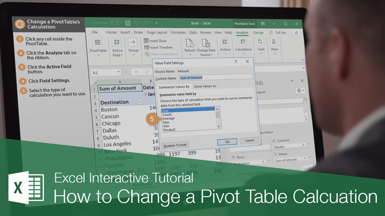
Now, let's watch how this is done in practice. The next video segment also demonstrates an extremely useful feature for MIS reports: showing values as a percentage.
Pivot Table Excel | Step-by-Step Tutorial
This video will demonstrate how to change the calculation type and how to show values as a percentage of the total—a very common reporting requirement.
Please watch two segments from the video: Changing the Summary Function (1:54 - 3:14): Watch how you can right-click the values to quickly change the summary from 'Sum of Sales' to 'Count' (number of sales) or 'Max' (the largest single sale). Showing Values as a Percentage (5:52 - 6:51): This is a key technique. Observe how you can add the 'Sales Amount' field to the Values area a second time, and then use the 'Show Values As' option to display it as a '% of Column Total'. This allows you to see both the absolute value and its contribution to the total.
Your Turn: Applying These Skills
Let's connect this to the types of reports you'll build as an MIS Executive. Using the same sales data, try to build the following summaries.
Scenario 1: Incident Analysis (Cybersecurity)
Imagine the data represents cybersecurity incidents. 'Salesperson' is the 'Analyst', 'Region' is the 'Incident Priority', and 'Sales' is the 'Data Volume (in GB)'.
Task: Create a PivotTable that shows, for each Analyst:
- The total number of incidents they handled. (Hint: Use a field in the Values area and set it to
Count). - The average data volume per incident. (Hint: Use the
Salesfield and set it toAverage). - Add a Filter for 'Incident Priority' (
Region) so you can view the report for only 'East' priority incidents.
Scenario 2: Performance Report (Recruitment)
Now, imagine 'Salesperson' is a 'Recruiter'.
Task: Create a PivotTable that shows a performance leaderboard:
- Put 'Recruiter' in the Rows area.
- Drag
Salesinto the Values area twice. - Leave the first one as
Sum of Sales. - Change the second one to show values as
% of Grand Total. Rename the column header to "% of Total Sales" for clarity.
Completing these short exercises will solidify your understanding of how to manipulate a PivotTable to answer specific business questions—a core function of any MIS role.
Conclusion
You've made a big leap forward today. You now have the skills to move beyond a basic summary and start building reports that are tailored to specific analytical needs.
Key Takeaways:
- You can build multi-dimensional reports by strategically using the Rows, Columns, and Filters areas.
- You can change the calculation in the Values area by right-clicking and selecting Summarize Values By to choose
Sum,Count,Average, and more. - For powerful comparison, you can add the same field to the Values area multiple times and use Show Values As to display metrics like
% of Grand Total.
In our next lesson, we will explore another essential feature for MIS reporting: grouping PivotTable data. You'll learn how to group dates into weeks, months, and years, and how to group numbers into ranges, allowing for even more powerful trend analysis.