Hello! Welcome to the first lesson in our module on summarizing data.
In your future role as an MIS Executive, you will constantly be asked to take large amounts of raw data and turn them into meaningful summary reports. Manually writing formulas for this is slow and error-prone. This is where PivotTables become your most powerful tool.
This lesson introduces PivotTables, focusing on the single most important step: creating one from a well-structured dataset. We'll build on what you learned about Excel Tables in Module 2 and see why they are the perfect foundation for creating dynamic, refreshable reports.
By the end of this session, you'll be able to take a large dataset and create a basic summary report in just a few clicks.
What is a PivotTable?
A PivotTable is an interactive tool that allows you to quickly summarize, or "pivot," large amounts of data. Instead of writing complex SUMIFS or COUNTIFS formulas, you can drag and drop data fields to see totals, counts, and averages grouped by different categories. For an MIS professional, this is the fastest way to answer questions like:
- "What were the total sales per region this month?"
- "How many incident tickets were closed by each team member?"
- "How many candidates are in each stage of the recruitment pipeline?"
The Golden Rule: Always Start with an Excel Table
In Module 2, you learned how to convert a range of data into a formal Excel Table. This is not just for formatting; it is the professional standard for preparing data for a PivotTable.
Why? When your data is in an Excel Table, your PivotTable is linked to the table's name, not a fixed range of cells (like A1:F500).
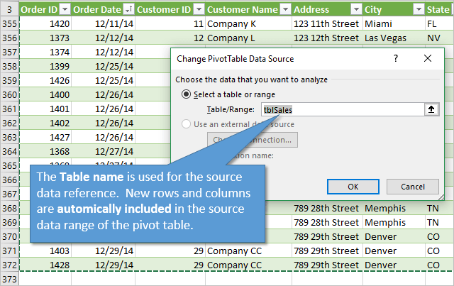
To see a great explanation of this principle in action, watch the first part of the following video.
Excel Pivot Table EXPLAINED in 10 Minutes (Productivity tips included!)
Leila Gharani provides a clear, concise explanation of why preparing your data as an Excel Table is a critical first step before creating a PivotTable.
Watch from the beginning until 2:42. Focus on the distinction between using a fixed range versus using a named Excel Table as the source for your PivotTable.
Creating Your First PivotTable: A Hands-On Guide
The best way to learn is by doing. We'll now walk through creating a PivotTable using a sample dataset.
This article from ExcelJet provides a clean, well-structured dataset perfect for practice. Please download the sample file before proceeding.
Follow the link in the 'Sample data' section of the article to download the Excel file named 'sample data for pivot table.xlsx'. Open the file and ensure you are on the 'Sales Data' sheet. Notice that the data is already formatted as an Excel Table.
Now that you have the file open, let's create a PivotTable to summarize total sales by region.
Step 1: Insert the PivotTable
With the sample file open, click on any single cell inside the data table. Go to the Insert tab on the ribbon and click the PivotTable button.
A "Create PivotTable" dialog box will appear.
- Table/Range: This should automatically show the name of our Excel Table (e.g.,
Table1). - Location: Choose "New Worksheet" to place your PivotTable on a new sheet, keeping your report separate from your raw data. This is standard practice.
Click OK.
Step 2: Understand the PivotTable Interface
You will now see a new, blank worksheet. On the left is the placeholder for your PivotTable report, and on the right is the PivotTable Fields pane. This pane is your control panel.
The list at the top of the pane shows all the column headers from your source data (Date, Color, Region, Units, Sales). The four boxes at the bottom are the areas where you will build your report:
- Rows: Fields placed here create the row labels of your report.
- Columns: Fields placed here create the column labels.
- Values: Fields placed here are what Excel will calculate (e.g., sum, count, average).
- Filters: Fields placed here allow you to filter the entire report.
For a visual walkthrough of these first steps, the following video is very helpful.
Pivot Table Excel | Step-by-Step Tutorial
Kevin Stratvert demonstrates the fundamental steps of inserting a PivotTable and introduces the PivotTable Fields pane.
Watch from 0:50 to 1:54. This covers inserting the PivotTable and familiarizing yourself with the field list and layout areas.
Step 3: Build a Simple Summary
Let's answer the question: "What are the total sales for each region?"
- In the PivotTable Fields pane, find the
Regionfield. - Click and drag
Regioninto the Rows area. You will see the regions (East, North, South, West) appear as row labels in your PivotTable on the left. - Next, find the
Salesfield. - Click and drag
Salesinto the Values area. Excel will automatically calculate the sum of sales for each region.
You have just created your first PivotTable! In under a minute, you have a summary report that would have otherwise required multiple SUMIF formulas.

Applying This to Your Experience
Think back to your work in recruitment or cybersecurity. You were often working with trackers containing large volumes of data. PivotTables are the perfect tool for summarizing that information for an MIS report.
For instance, in a recruitment tracker, you might have columns for Candidate Name, Status (e.g., "Screening," "Interview," "Hired," "Rejected"), and Recruiter.
How to Create a Recruitment Tracker in Excel
This blog post shows how to apply the exact technique you just learned in a recruitment context. You don't need to build it now, just read this short section to see the direct application.
Read the section 'Summarize Your Data with a PivotTable'. Notice how they drag 'Status of Application' to the Rows area and 'Candidate Name' to the Values area (which defaults to 'Count of Candidate Name') to instantly see how many candidates are in each stage.
This simple summary is the first step in building the recruitment pipeline reports and dashboards we will tackle in the final modules of this course.
Conclusion
In this lesson, you've learned the fundamental and most crucial skill in data summarization: creating a PivotTable.
Key Takeaways:
- PivotTables are Excel's most powerful tool for quickly summarizing large datasets without formulas.
- The best practice is to always base your PivotTable on data formatted as an Excel Table to ensure your reports are dynamic and easy to update.
- You build a PivotTable by dragging fields from your source data into the Rows, Columns, and Values areas of the PivotTable Fields pane.
You've successfully created a basic summary report. In our next lesson, we will explore how to configure PivotTable fields in more detail. You will learn how to change the calculation type (e.g., from Sum to Count or Average), add multiple layers of data to your rows and columns, and build more sophisticated summary reports.