Calculating IRR for Simple Projects

The IRR Equation: The Root of the Problem

As a quick refresher, the IRR, which we'll call $i^{\ast }$, is the rate that satisfies this equation:

Where $C{F}_t$ is the cash flow at time $t$ and $N$ is the project's life.

For a project with an initial cost $P$ and a series of future inflows $F_t$, the equation looks like this:

This is a polynomial equation of degree $N$ in terms of the variable $x=\frac{1}{1+i^{\ast }}$. For any project longer than two or three periods, solving this equation directly for $i^{\ast }$ becomes impractical or impossible by hand. This is why we need other methods.

The following reading sets up a typical problem and introduces the methods we will explore.

As the text points out, we need a systematic way to find the answer. Let's look at a few methods, starting with the simplest case.

Method 1: Direct Solution for Simple Projects

For very simple projects, we actually can solve for the IRR directly. This is generally limited to projects with only two or three cash flows.

Let's recap the key takeaway from Case A:

Project: Invest $2,000 today ($P$), receive $3,500 in 4 years ($F$).
Equation:

Solution: By rearranging the equation, you can directly solve for $i^{\ast }$.

This direct method is quick and easy when it applies, but most of your real-world projects, like developing a new software feature with annual returns, will have more complex cash flows.

Method 2: Trial and Error (The Iterative Approach)

This is the most fundamental and intuitive method for finding the IRR of any project by hand. The process is a systematic search for the rate that drives the NPW to zero.

The logic relies on the relationship between the discount rate and the NPW:

• As the discount rate increases, the present value of future inflows decreases, thus the NPW decreases.
• As the discount rate decreases, the present value of future inflows increases, thus the NPW increases.

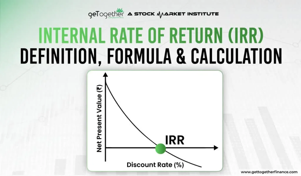
This relationship gives us a clear strategy for our search:

1. Guess an interest rate, $i$.
2. Calculate the NPW using this rate.
3. If NPW > 0, your guess for $i$ was too low. Try a higher rate.
4. If NPW < 0, your guess for $i$ was too high. Try a lower rate.
5. Repeat until the NPW is very close to zero.

Let's see this in action.

The example demonstrates the process perfectly. Starting with a guess of 5% yields a positive NPW ($985.61), so the next guess must be higher. Guessing 10% yields a negative NPW (-$91.76). This tells us the true IRR is bracketed between 9% and 10%. The process then refines the guess within that range until it lands on an NPW very close to zero, giving an IRR of approximately 9.53%.

A Refinement: Linear Interpolation

Once you have bracketed the IRR between two rates (one giving a positive NPW and one a negative), you can use linear interpolation to get a very close estimate without further guessing.

The formula is:

Where:

• $i_L$ = The lower interest rate guess (which gives a positive NPW).
• $i_H$ = The higher interest rate guess (which gives a negative NPW).
• ${\text{NPW}}_L$ = The positive NPW at $i_L$.
• ${\text{NPW}}_H$ = The negative NPW at $i_H$.

Using the values from the resource's example:

• $i_L=9\%$, ${\text{NPW}}_L=\$107.51$
• $i_H=10\%$, ${\text{NPW}}_H=-\$91.76$

This is a very fast way to get an accurate estimate.

The Modern Approach: Using Software

Given your background in software engineering, it's important to note that while understanding the manual method is crucial for conceptual clarity, you will rarely perform trial-and-error calculations in practice.

Modern tools automate this process.

• Spreadsheets: Microsoft Excel and Google Sheets have a built-in IRR() function. You simply provide the range of cash flows, and it instantly returns the IRR.
• Programming: In Python, the NumPy library has a function, numpy.irr(), that does the same thing.

These tools use sophisticated numerical algorithms (like the Newton-Raphson method) to perform the iteration and find the root of the NPW equation almost instantly. Learning the manual method ensures you understand exactly what these functions are accomplishing under the hood.

Conclusion

Today, we've moved IRR from a theoretical concept to a number we can actually calculate. While it can't always be solved for directly, we have a robust iterative method to find it.

• Key Takeaways:
  • Finding the IRR means solving the NPW=0 equation for the interest rate $i^{\ast }$.
  • For most projects, this equation is a high-degree polynomial that cannot be solved directly.
  • Trial and error is the fundamental manual method: guess a rate, calculate NPW, and systematically adjust your guess based on whether the NPW is positive or negative.
  • Linear interpolation is a useful shortcut to quickly estimate the IRR once it's been bracketed between two rates.
  • In a professional setting, you will use software functions like IRR() in Excel or numpy.irr() in Python, which automate the trial-and-error process.

Preview of the Next Lesson

Now that we can define IRR and calculate it, the next step is to formalize its use in decision-making. In the next lesson, we will focus on how to evaluate project acceptability by comparing its IRR to the MARR, solidifying the simple but powerful decision rule we introduced earlier.