Decision Tree Analysis for Real Options

Introduction

In our previous lesson, we established a crucial strategic concept: real options. We defined what they are—the right, but not the obligation, to take actions like deferring, abandoning, or expanding a project—and identified how they manifest in technology investments. You learned that this flexibility has immense value, especially in the uncertain environments you navigate as a software developer and manager.

However, simply identifying an option isn't enough. To make a sound investment decision, you need to quantify its worth. Today's lesson directly addresses that challenge and fulfills the learning outcome: Use decision tree analysis to model and evaluate a project that includes a real option. We will move from the "what" to the "how much" by learning a powerful technique to map out and financially analyze projects with embedded flexibility. This method provides a formal structure for the sequential decision-making you already practice intuitively.

1. Visualizing Decisions: An Introduction to Decision Trees

At its heart, a decision tree is a flowchart that maps out a project's possible pathways. It visualizes the sequence of your decisions, the uncertain events that can occur, and the financial outcome of each path.

This approach explicitly corrects a major flaw in standard Net Present Worth (NPW) analysis, which assumes a passive, fixed path from start to finish.

As the text highlights, decision trees bring your strategic choices to the forefront. Let's look at the basic components.

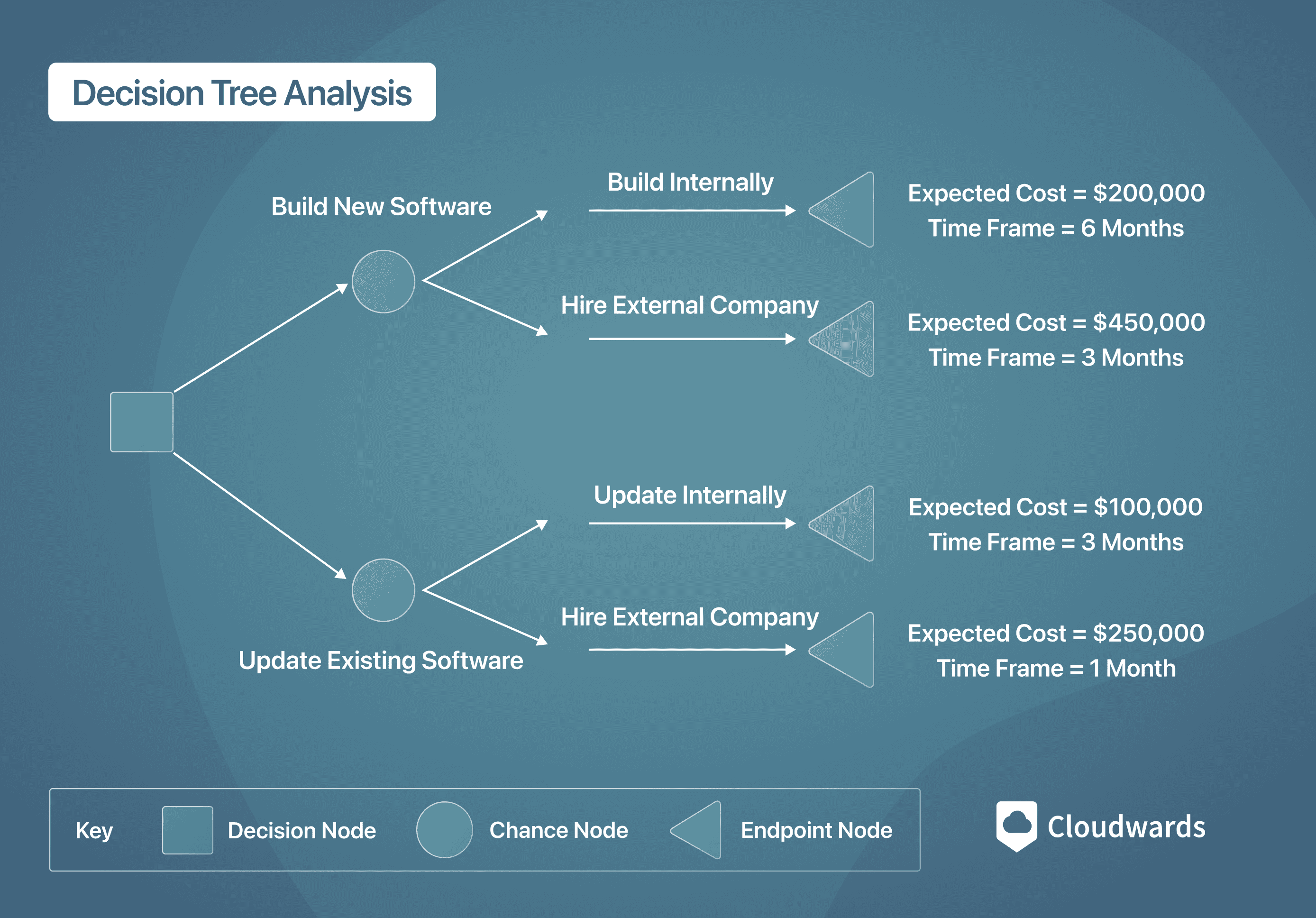
Here are the key elements you need to know:

• Decision Nodes (Squares): Points in time where you, the manager, must make a choice. In the image, the first decision is "Build New Software" or "Update Existing Software."
• Chance Nodes (Circles): Points where an uncertain event occurs, outside of your direct control. Each possible outcome has an estimated probability. For example, a chance node could represent whether market demand turns out to be "High" (60% probability) or "Low" (40% probability).
• Branches: These are the lines connecting the nodes. Branches extending from a decision node represent your choices, while branches from a chance node represent possible outcomes of an uncertain event.
• Terminal Nodes (Triangles): These are the endpoints of each possible path. Each terminal node has a final payoff or cost associated with it—this is the NPW of that specific scenario.

2. Valuing Flexibility: The Rollback Method

The true power of a decision tree lies in its analysis. How do you use this map to find the best strategy and the project's total value? You use a technique called rollback or backward induction.

The logic is simple: to make the best decision today, you must first know the value of all possible future positions. Therefore, you start at the end of the tree (the final outcomes) and work your way backward to the beginning.

Let's walk through this process using a practical example of a technology migration project with an embedded option to defer and an option to abandon.

Now, let's analyze the tree from that example using the rollback method. The calculations can look complex, but the logic is straightforward. We'll follow the step-by-step breakdown provided in the resource.

Let's summarize the rollback process you just read about:

1. Start at the End: Begin at the terminal nodes (the final outcomes in 2010 or 2011). These have known cash flow values (e.g., CHF 79.4M for success, CHF 7.9M for salvage).

2. Move to a Chance Node: To find the value at a preceding chance node, calculate the expected value. You do this by multiplying the value of each outcome by its probability and summing the results. Then, discount this expected value back one period.

   • For example, the value at Node A (in 2009) is the probability-weighted value of the 2010 outcomes, discounted back one year, minus the investment cost for that stage.
     $\text{Value at A}=\frac{(P_{success}\times {\text{CF}}_{success})+(P_{failure}\times {\text{CF}}_{salvage})}{1+r}-\text{Investment}$

3. Move to a Decision Node: When you roll back to a decision node, you apply the core rule of option valuation: choose the branch with the highest value.

   • For instance, if you're at a node where you can either "Abandon" (for a value of 0) or "Proceed" (with an expected value of CHF 48.7M), the decision is clear. You choose to proceed. The value of the decision node is the value of the best available choice.

4. Repeat to Time 0: Continue this process of calculating expected values at chance nodes and picking the best path at decision nodes until you arrive back at the very first node (time 0).

The final value at the root of the tree (CHF 26.8M in the example) is the project's NPW, including the value of all the embedded options. As the paper concludes, the value of the option itself can be found by comparing the NPW with flexibility (CHF 26.8M) to the NPW without flexibility (CHF 27.2M). In that specific case, the option to wait actually had a negative value, demonstrating that flexibility isn't always beneficial if it causes costly delays.

3. A More Advanced Model: Binomial Trees

Decision trees are powerful, but the probabilities can be subjective. A more structured approach used in real options analysis is the binomial tree (or lattice). It models the value of the underlying asset (the completed project) as evolving through a series of "up" or "down" movements over time.

This model is a natural fit for your software background. You can think of the time steps (δt) as project phases or even agile sprints. At the end of each step, the project's potential value has either gone up or down, and you have an option to continue, abandon, or change course.

Let's examine a detailed example that uses a binomial tree to compare an agile project (with an abandon option) to a traditional plan-driven project.

The key takeaways from this binomial tree example are:

• Valuing the Abandon Option: In Figure 2 (the agile project), look at the nodes where the option value is circled (e.g., at t5, the bottom two nodes have a value of 65). This is where the rollback analysis determined that abandoning the project for its salvage value (65M) was more valuable than continuing. The tree visually shows you exactly when and under what conditions the option should be exercised.
• Comparing Strategies: The initial value of the agile project (with the option) at t1 is $106M. The value of the plan-driven project (without the option) is $100M. The difference of $6M is the calculated value of the flexibility provided by the abandon option.
• Connecting to Agile: This model beautifully quantifies a core benefit of agile development. By delivering value incrementally (modularity) and having clear decision points (early termination), you create real options that limit downside risk and have quantifiable economic value.

Conclusion

Today, we've moved real options from a theoretical concept to a practical evaluation tool. You've learned how to structure complex, uncertain projects using decision trees and how to analyze them to find the most valuable strategic path.

• Key Takeaways:
  • Decision Tree Analysis (DTA) is a method to model and visualize sequential decisions and uncertain events over time.
  • The rollback method is used to analyze a decision tree by starting at the final outcomes and working backward, calculating expected values at chance nodes and choosing the best path at decision nodes.
  • The value found at the start of the tree is the project's NPW, inclusive of the value of its embedded managerial flexibility (real options).
  • More advanced binomial trees use a similar rollback logic but model uncertainty as a series of up/down movements in the underlying asset's value, providing a robust way to value options like the option to abandon.

Preview of the Next Lesson

We have now seen what a real option is and how to value one using decision trees. In our next lesson, we will synthesize these ideas. We will formally discuss how real options analysis can capture strategic value missed by traditional NPV, solidifying why this modern approach is so critical for evaluating the high-uncertainty, high-flexibility technology projects you lead.