Hello! Welcome back to our module on managing project uncertainty.
In our last lesson, we explored the purpose of sensitivity analysis. We learned that it's a strategic tool used to identify the project variables that pose the biggest risks to our financial success, telling us where to focus our efforts to "buy down" uncertainty.
Today, we move from the "why" to the "how." Our goal is to perform a one-variable sensitivity analysis on a project's Present Worth (PW). We'll walk through the mechanics of this process using a clear, numerical example. This will give you a concrete method for assessing how sensitive your software or technology project's value is to the forecasts you make.
1. Establishing the Base Case
Before we can test for sensitivity, we need a baseline. Every sensitivity analysis begins with calculating the project's Present Worth (or Net Present Value, NPV) using your most likely estimates for all variables. This is the base case against which all variations will be compared.
Let's work with a tangible example.
Accounting for Uncertainty with Sensitivity Analysis
The following document from CPA Ireland, titled 'The Investment Decision – Accounting for Uncertainty with Sensitivity Analysis', provides a clear, step-by-step example. We will use this case study throughout the lesson.
Please read the 'Introduction' and the first part of '2.0 Sensitivity Analysis Explained'. Focus on understanding the setup of the investment opportunity for ABC Ltd and how its base-case NPV of €549,200 is calculated. You can stop when you see the heading '2.1 Realistic Deviation'.
As you saw, the base case is a standard Present Worth calculation, just like we've done in previous modules. It involves:
- An initial investment (outflow) at Year 0.
- A series of annual net cash flows, calculated from revenues (demand x price) and costs (variable and fixed).
- Discounting those future cash flows back to the present using the cost of capital (10%) to find the NPV.
This base case of €549,200 tells us the project is acceptable if all our forecasts are correct. Now, let's test that assumption.
2. Performing the Analysis: Two Common Methods
With our base case established, we can now systematically vary our key inputs one at a time. This is the core of one-variable sensitivity analysis. We will look at two popular ways to do this.
Method 1: Analyzing Realistic Deviations
One straightforward approach is to define a plausible range for each variable. You estimate a realistic "unfavorable" (pessimistic) and "favorable" (optimistic) value for each key input and then recalculate the project's PW for each scenario.
Accounting for Uncertainty with Sensitivity Analysis
Let's continue with the CPA Ireland document to see how this method is applied.
Read the section titled '2.1 Realistic Deviation'. Pay close attention to Table 1, which shows the deviations, and Table 2, which shows the resulting NPVs. Notice how for each calculation, only one input is changed from the base case.
The output of this analysis is a table showing the range of possible PW outcomes for each variable.
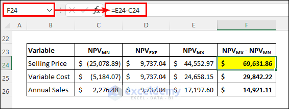
By looking at the range of NPVs in Table 2 of the document, you can immediately get a feel for the most critical variables. An unfavorable deviation in "Equipment Cost" or "Demand in Units" pushes the NPV into negative territory, making them high-risk variables. In contrast, even the unfavorable case for "Variable Cost per Unit" results in a positive NPV, suggesting it's a lower-risk variable.
Test your understanding!
Using the data from the ABC Ltd example, calculate the project's NPV if the selling price per unit has an unfavorable deviation to €190, while all other variables remain at their forecast (base case) values. Does the project remain viable?
(Recall: 5-year project, 10% cost of capital, PVAF is 3.791)
Show answer
- New Revenue: 10,000 units * €190/unit = €1,900,000
- New Annual Net Cash Flow: €1,900,000 (Revenue) - €400,000 (Variable Costs) - €400,000 (Overheads) = €1,100,000
- New PV of Annual Cash Flows: €1,100,000 * 3.791 = €4,170,100
- New NPV: €4,170,100 - €4,000,000 (Initial Investment) = €170,100
Yes, the project remains viable (NPV is positive), which matches the result in Table 2 of the resource.
Method 2: Calculating the Margin of Safety
A second, more precise method is to calculate the margin of safety. This tells you the exact percentage change in a variable that will drive the project's PW down to zero. This is essentially a breakeven calculation for each input variable.
Accounting for Uncertainty with Sensitivity Analysis
The CPA document also explains this second method.
Please read section '2.2 Margin of Safety'. Focus on understanding the concept and the formula. Note how a smaller margin of safety implies a more sensitive, higher-risk variable.
As shown in Table 3 of the resource, the selling price has a margin of safety of only -7.25%. This means a mere 7.25% drop in price from the forecast would make the project financially unviable. In contrast, the variable cost has a margin of safety of 36.2%, meaning it could increase by over a third before the project breaks even. This confirms that selling price is a far more sensitive variable than variable cost for this project.
3. Automating the Analysis with Spreadsheets
While you can perform these calculations manually for simple projects, it becomes tedious quickly. In practice, sensitivity analysis is almost always performed using spreadsheet software like Microsoft Excel or Google Sheets.
Your background as a software engineer means you already appreciate the importance of building robust models. The key is to set up your spreadsheet with all inputs in a separate area, and then build your cash flow and PW calculations using formulas that reference those input cells. Never hard-code input values directly into formulas.
Once your model is set up this way, you can use built-in tools to automate the sensitivity analysis.
ESD.70J / 1.145J Engineering Economy Module
This short clip from an MIT lecture on Engineering Economy demonstrates how to use the 'Data Table' feature in Excel to perform a one-variable sensitivity analysis. It shows how to automatically generate the output table we've been discussing.
Watch the segment that explains and demonstrates the 'One-way Data Table'. It starts around slide 29 and goes for a few slides. Focus on the concept of setting up a column of input values and having Excel automatically fill in the corresponding output values (in this case, the difference in NPV between two plans).
Using a data table automates the repetitive process of changing an input and recording the output, allowing you to quickly analyze the sensitivity of your project's PW to dozens of different values for a key variable.
Conclusion
Today, you've learned the practical steps for conducting a one-variable sensitivity analysis. This is a fundamental skill for evaluating the risk profile of any technology project.
- Key Takeaways:
- Sensitivity analysis always starts with a base case calculation of Present Worth using your best-guess estimates.
- The core process involves changing one variable at a time while holding others constant.
- The "Realistic Deviation" method helps you see the range of possible outcomes by testing optimistic and pessimistic scenarios for each variable.
- The "Margin of Safety" method calculates the percentage change required for a variable to make the project's PW equal zero, directly quantifying its sensitivity.
- Properly structured spreadsheets with tools like Data Tables are essential for performing this analysis efficiently.
Preview of the Next Lesson
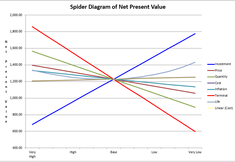
We have now generated a lot of numerical data. But how do we communicate these findings clearly to stakeholders? In our next lesson, we will learn how to interpret the results of a sensitivity analysis using a spider diagram, a powerful visualization tool that shows the relative sensitivity of all variables at a single glance.