Linear Regression with Scikit-learn: Fitting and Interpretation

Introduction

In our last session, we established the core principle of linear regression: finding a "best-fit" line by minimizing the Sum of Squared Errors (SSE). We saw that the model is represented by the equation $\hat{y}={\beta }_0+{\beta }_{1}x$ and that training the model means finding the optimal values for the intercept (${\beta }_0$) and the coefficient (${\beta }_1$).

Today, we move from theory to practice. You will learn how to fit a linear regression model using scikit-learn and interpret its coefficients. This lesson is all about implementation and understanding what the model tells us once it's trained—a direct application of the concepts we've discussed.

Implementing Linear Regression with Scikit-Learn

Let's dive straight into the code. The process involves preparing your data, creating a model instance, and then "fitting" it to the data. The video below provides a hands-on walkthrough. While the video generates its own data, the steps are universal.

As you saw, the process in scikit-learn is remarkably straightforward:

1. Prepare Data: Separate your features (the independent variables, X) from your target (the dependent variable, y). It's standard practice to split this data into training and testing sets, as shown in the video, to evaluate the model's performance on unseen data.
2. Create a Model: Instantiate the LinearRegression class: model = LinearRegression().
3. Fit the Model: Train the model by calling the .fit() method with your training data: model.fit(X_train, y_train).

This .fit() method is where scikit-learn performs the Ordinary Least Squares (OLS) optimization we discussed, finding the $\beta$ values that minimize the sum of squared errors.

For a comprehensive text-based guide that covers these steps, you can refer to the "Real Python" article on Linear Regression.

Interpreting the Model's Coefficients

Once the model is fitted, scikit-learn stores the learned parameters—the intercept (${\beta }_0$) and coefficient(s) (${\beta }_1,{\beta }_2,...$)—as attributes of the model object.

• The intercept is stored in .intercept_.
• The coefficient(s) are stored in .coef_.

But what do these numbers actually mean?

Let's crystallize those definitions:

• Intercept (.intercept_): This is the predicted value of your target variable ($y$) when all your input features ($X$) are equal to zero.
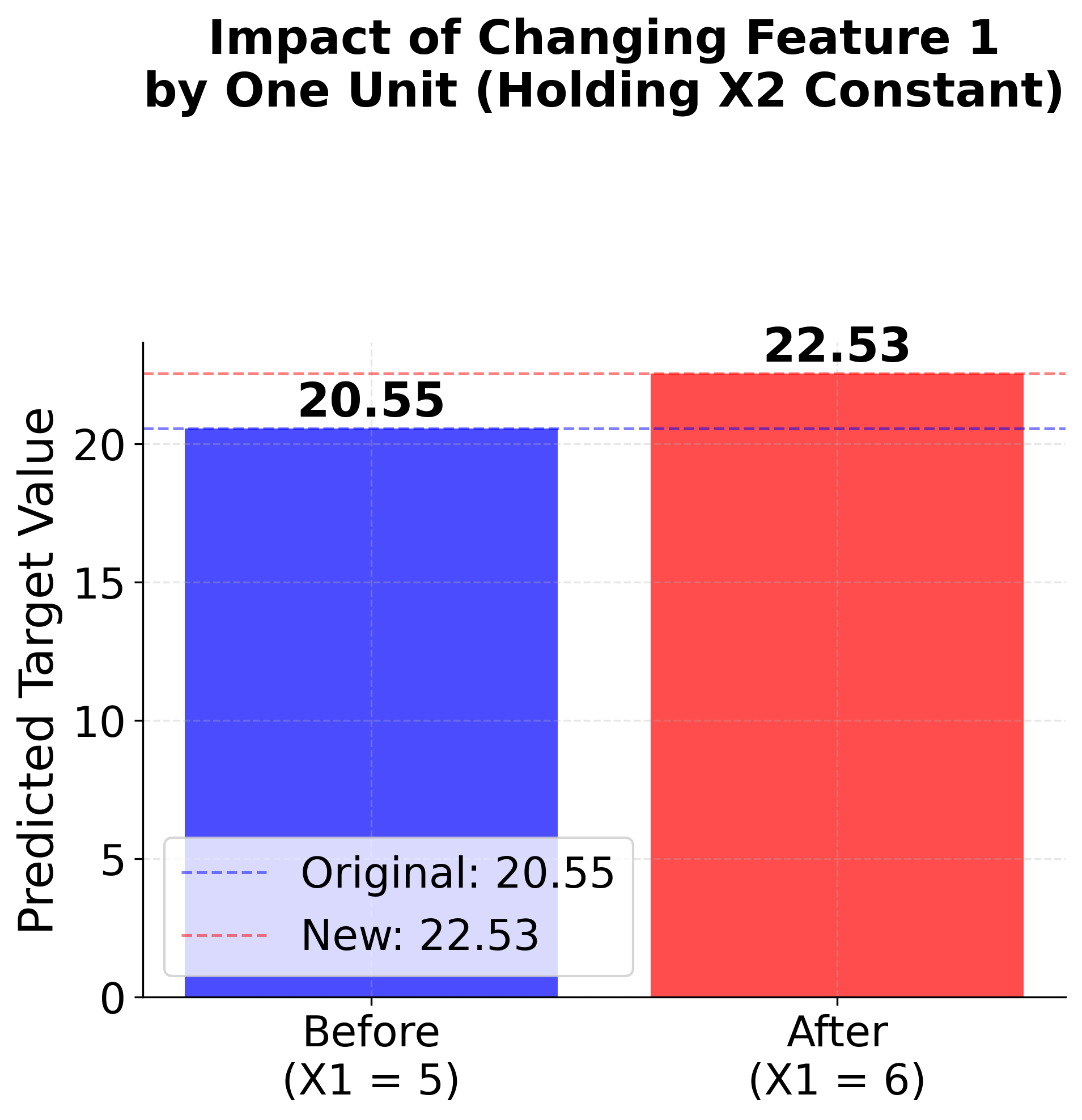
• Coefficient (.coef_): This represents the change in the predicted target variable for a one-unit increase in the corresponding feature, assuming all other features are held constant.

For a simple linear regression with one feature, the coef_ is a single value (the slope). For multiple linear regression, it's an array, with one value for each feature.

This image provides a great visual intuition for what a coefficient represents.

From Simple to Multiple Linear Regression

The concept extends seamlessly to multiple linear regression, where you use multiple features to predict a target. The equation simply includes more terms:

The beauty of scikit-learn is that the code remains almost identical. You just provide an X with multiple columns. The resulting .coef_ attribute will be an array of coefficients, one for each feature.

A Crucial Caveat: The Role of Feature Scaling

When interpreting coefficients from a multiple regression model, it's tempting to assume that the feature with the largest coefficient is the "most important." This is often incorrect.

The magnitude of a coefficient depends on the scale of its feature. A feature measured in days (e.g., age_in_days) will have a much smaller coefficient than the same feature measured in years (age_in_years), even though their predictive impact is identical.

To compare the importance of features based on their coefficients, you must first bring them to a common scale. We covered this with StandardScaler in our first module, and this is a prime example of where it becomes essential.

Conclusion

You've now bridged the gap between the theory of OLS and its practical application. You can build a linear regression model and, just as importantly, make sense of what it has learned.

Key Takeaways:

• You can fit a linear regression model in scikit-learn using LinearRegression().fit(X, y).
• The learned intercept (.intercept_) is the model's baseline prediction when all features are zero.
• Each coefficient in .coef_ represents the predicted change in the target for a one-unit increase in its corresponding feature, holding all other features constant.
• Directly comparing the magnitudes of coefficients to judge feature importance is misleading unless the features have been scaled first.

Preview of the Next Lesson

Our model finds the best fit for the training data, but how well does it generalize to new, unseen data? In the next lesson, we will explore the fundamental concepts of bias and variance and their trade-off. This will set the stage for understanding overfitting and why more complex models aren't always better.