Least Squares Regression

Introduction

In the previous modules, we explored unsupervised learning, where our goal was to find hidden patterns in data without any pre-defined labels, like with K-Means and GMMs. We're now shifting gears to supervised learning. Here, the dataset includes a specific target variable we want to predict. Our goal is to build a model that learns the mapping from input features to this target.

This week, we start with one of the most fundamental supervised learning algorithms: Linear Regression. It's used for regression tasks, where the goal is to predict a continuous numerical value—like the price of a house, the temperature tomorrow, or the weight of a person.

Today's learning outcome is to formulate linear regression as a model that minimizes the sum of squared errors. We'll focus on the core principle that defines how a linear regression model finds the "best-fit" line for a set of data.

The Linear Regression Model

At its heart, linear regression assumes a linear relationship between the input features and the target variable. For a simple case with one input feature ($x$) and one target variable ($y$), this relationship is represented by the familiar equation of a straight line.

The following short video clearly introduces this equation and the terminology used in machine learning.

As the video explained, our model's prediction, which we'll call $\hat{y}$ ("y-hat"), is given by:

• $x$: The input feature (e.g., square footage of a house).
• $\hat{y}$: The predicted value (e.g., predicted price of the house).
• ${\beta }_1$: The coefficient or weight associated with the feature $x$. It represents the slope of the line—how much $\hat{y}$ changes for a one-unit change in $x$.
• ${\beta }_0$: The intercept or bias. It's the value of $\hat{y}$ when $x$ is zero.

The goal of "training" a linear regression model is to find the optimal values for ${\beta }_0$ and ${\beta }_1$ that make our line fit the data as closely as possible. But how do we define "closely"?

Measuring Error: The Sum of Squared Errors (SSE)

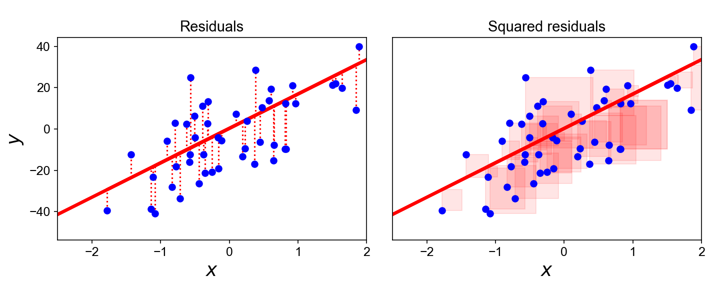
Imagine plotting your data points and drawing a random line through them. Some points will be above the line, some below. The vertical distance between each data point and the line is our error, or more formally, the residual.

Where $y_i$ is the actual, true value for the i-th data point.

To get a single number that represents the total error for the entire dataset, we can't just sum up the residuals, because positive and negative errors would cancel each other out. The standard solution is to square each residual and then sum them all up. This gives us the Sum of Squared Errors (SSE).

The next video provides an excellent, intuitive explanation of this entire process.

The process described in the video—finding the line that has the least sum of squares—is exactly why the most common method for linear regression is called Ordinary Least Squares (OLS).

The image below provides a static visual that summarizes this concept perfectly. The vertical lines are the residuals, and the colored squares represent the squared residuals. The goal of OLS is to adjust the line to make the total area of all those squares as small as possible.

Formalizing the Objective

We've built the intuition, so now let's put it into a formal objective. Linear regression is an optimization problem where we want to find the parameters (${\beta }_0,{\beta }_1$) that minimize our cost function, which is the SSE.

To summarize the key points from the reading:

1. The Objective Function: We are trying to solve the following:

   $$\underset{{\beta }_0,{\beta }_1}{\min }\sum _{i=1}^n(y_i-{\hat{y}}_i{)}^2$$

   This is just the mathematical way of saying "find the ${\beta }_0$ and ${\beta }_1$ that result in the minimum Sum of Squared Errors."

2. Why Square the Errors?

   • Penalizes Large Errors: A data point that is far from the line contributes much more to the total error than a point that is close, encouraging the model to pay more attention to large mistakes.
   • Mathematical Convenience: The squared error function is smooth and has a single global minimum. This allows for efficient optimization, for example using calculus (taking derivatives to find the minimum) or iterative methods like gradient descent, which you may be familiar with from your work with neural networks.

Conclusion

In this lesson, we made the transition to supervised learning and established the foundational principle of linear regression.

Key Takeaways:

• Linear regression models a linear relationship between features ($x$) and a continuous target ($y$) using the equation $\hat{y}={\beta }_0+{\beta }_{1}x$.
• The "best" line is the one that minimizes the total error between the model's predictions (${\hat{y}}_i$) and the actual data ($y_i$).
• We quantify this total error using the Sum of Squared Errors (SSE), which is the sum of all the squared vertical distances (residuals) from each point to the line.
• The process of finding the model coefficients (${\beta }_0,{\beta }_1$) that minimize the SSE is called Ordinary Least Squares (OLS).

Preview of the Next Lesson

Now that you understand the objective of linear regression, the next step is to put it into practice. In our next lesson, you will fit a linear regression model using scikit-learn and interpret its coefficients. We will take the concepts from today and apply them to a real dataset.