GMM vs. K-Means: Soft vs. Hard Clustering in Scikit-learn

Introduction

In our last session, we demystified the "engine" behind Gaussian Mixture Models: the Expectation-Maximization (EM) algorithm. We established that EM is an iterative process that cleverly solves the "chicken-and-egg" problem of finding cluster parameters by alternating between an Expectation step (calculating probabilistic assignments, or "responsibilities") and a Maximization step (updating cluster parameters).

Today, we transition from theory to practice. Our goal is to fit a GMM using scikit-learn and compare its probabilistic assignments to K-means' hard assignments. You'll see firsthand how GMM's "soft" clustering provides a more nuanced understanding of your data compared to the rigid assignments of K-means.

K-Means vs. GMM: Hard vs. Soft Clustering

Before we dive into the code, let's crystallize the fundamental difference between K-means and GMM.

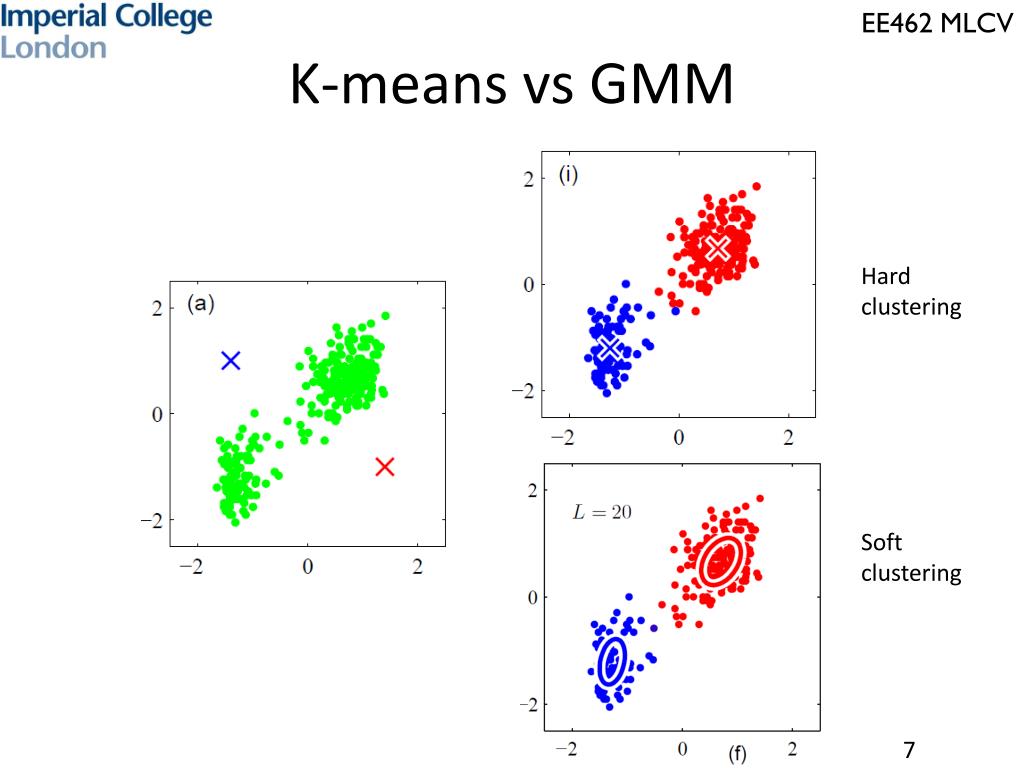
• K-Means performs hard clustering. It assigns each data point to exactly one cluster. The boundaries between clusters are sharp.
• GMM performs soft clustering. It calculates the probability that a data point belongs to each of the clusters. This is a more flexible approach, especially when clusters overlap or have non-spherical shapes.

This short video provides a concise summary of these differences.

The image below provides a great visual for this concept. On the left (K-means), every point is either 100% blue or 100% red. On the right (GMM), points in the overlapping region can be a mix, reflecting the uncertainty of their assignment. The ellipses also show that GMM has learned the shape and orientation of the clusters, not just their centers.

Fitting a GMM with Scikit-Learn

Now, let's see how this is done in practice. You are already familiar with the scikit-learn API, so you'll find fitting a GMM to be very straightforward. The key methods are:

• .fit(X): Trains the GMM on the data X using the EM algorithm.
• .predict(X): Provides the "hard" cluster assignment for each data point (i.e., the cluster with the highest probability).
• .predict_proba(X): Provides the "soft" cluster assignments—a matrix where each row corresponds to a data point and each column is the probability of that point belonging to a cluster.

The following video demonstrates this entire workflow, from generating data to fitting the model and interpreting the probabilistic outputs.

Code in Action: A Direct Comparison

Let's put KMeans and GaussianMixture side-by-side with a code snippet. You can run this in a Jupyter Notebook or Google Colab environment to see the difference in their outputs directly.

We will generate two slightly overlapping clusters. Notice how the outputs of kmeans.labels_ and gmm.predict() are single integer labels, while gmm.predict_proba() gives a richer, probabilistic view.

import numpy as np
from sklearn.cluster import KMeans
from sklearn.mixture import GaussianMixture
from sklearn.datasets import make_blobs




# 1. Generate synthetic data with some overlap
X, y_true = make_blobs(n_samples=300, centers=2, cluster_std=1.5, random_state=42)




# --- K-Means (Hard Clustering) ---
kmeans = KMeans(n_clusters=2, random_state=42, n_init=10)
kmeans.fit(X)
kmeans_labels = kmeans.labels_

print("--- K-Means Hard Assignments ---")
print("Labels for the first 5 points:")
print(kmeans_labels[:5])
print("-" * 30)





# --- GMM (Soft and Hard Clustering) ---
gmm = GaussianMixture(n_components=2, random_state=42, n_init=10)
gmm.fit(X)




# Get the hard assignments from GMM
gmm_hard_labels = gmm.predict(X)




# Get the soft (probabilistic) assignments
gmm_soft_labels = gmm.predict_proba(X)

print("\n--- GMM Hard Assignments ---")
print("Labels for the first 5 points (from .predict()):")
print(gmm_hard_labels[:5])
print("-" * 30)

print("\n--- GMM Soft/Probabilistic Assignments ---")
print("Probabilities for the first 5 points (from .predict_proba()):")



# Using np.round for cleaner output
print(np.round(gmm_soft_labels[:5], 3))
print("-" * 30)




# Example: Find a point with high uncertainty
# A point is uncertain if its max probability is not close to 1.0
uncertainty = 1 - gmm_soft_labels.max(axis=1)
most_uncertain_point_idx = np.argmax(uncertainty)

print("\n--- Analyzing an Uncertain Point ---")
print(f"Point with highest uncertainty is at index: {most_uncertain_point_idx}")
print("Its probabilities are:", np.round(gmm_soft_labels[most_uncertain_point_idx], 3))
print("K-Means assigned it to cluster:", kmeans_labels[most_uncertain_point_idx])
print("This nuance is lost with hard clustering!")

When you run this code, pay attention to the output for the "uncertain point." You'll see that GMM assigns it probabilities like [0.55, 0.45], indicating it lies in an ambiguous region. K-means, by contrast, is forced to choose one cluster, masking this valuable uncertainty information.

For a more detailed written guide on using GaussianMixture in scikit-learn, including explanations of its parameters, the article "Gaussian Mixture Models (GMMs): from Theory to Implementation" is an excellent resource. The section titled GMM in Scikit-Learn is particularly relevant.

Conclusion

Congratulations! You've successfully moved from the theory of GMMs and EM to practical implementation.

Key Takeaways:

• You can fit a GMM using the sklearn.mixture.GaussianMixture class, which uses the EM algorithm under the hood.
• K-means provides hard assignments: each point belongs to exactly one cluster (.labels_).
• GMMs provide soft assignments: each point has a probability of belonging to every cluster (.predict_proba()). This is the key advantage of GMMs.
• The probabilistic output from a GMM is valuable for understanding uncertainty and handling complex, overlapping cluster structures.

Preview of the Next Lesson

This lesson concludes our exploration of unsupervised learning for this course. We will now pivot to Supervised Learning, where the goal is to predict a specific target value based on input features. Our first topic will be Linear Regression, a foundational algorithm for predicting continuous values. We will start by formulating linear regression as a problem of minimizing the sum of squared errors.