Equilibrium: Schedules & Graphs

Hello! Welcome to the next lesson in your CFA Level 1 Economics course.

Introduction

In our previous lessons, we built the foundational tools of microeconomics: the demand curve and the supply curve. We defined them, understood the laws of demand and supply, and cataloged the various non-price factors that cause each curve to shift.

Now, it's time to bring these two concepts together. This lesson focuses on the learning outcome: to determine equilibrium price and quantity from demand and supply schedules or graphs. We will explore how the interaction of buyers (demand) and sellers (supply) in a market leads to a state of balance, known as equilibrium. We will identify this point on a graph, in a data table (a schedule), and finally, by using simple algebra—a method that leverages your mathematical background for a more precise understanding.

1. Understanding Market Equilibrium

At its core, a market's purpose is to bring buyers and sellers together. But at what price will they trade, and how much will be exchanged? The answer lies in the concept of equilibrium. Market equilibrium occurs at the price and quantity where the plans of consumers and the plans of producers agree. In other words, it's the point where the quantity of a good that buyers are willing and able to purchase is exactly equal to the quantity that sellers are willing and able to sell.

This video from Khan Academy provides an excellent, intuitive explanation of how a market reaches equilibrium. It also demonstrates what happens when the market is out of balance, leading to either a shortage or a surplus.

Market equilibrium | Supply, demand, and market equilibrium | Microeconomics | Khan Academy

Please watch this video, 'Market equilibrium'. It visually demonstrates how the demand and supply curves interact to establish an equilibrium price and quantity. Pay close attention to the concepts of 'shortage' and 'surplus' and how the market naturally adjusts back to equilibrium.

Watch the full video (from 00:00 to 10:14). It will walk you through setting up the graph, analyzing what happens when the price is too low or too high, and finally defining the equilibrium point.

As the video explained, let's formalize these key concepts:

Equilibrium: The point where the supply and demand curves intersect.
Equilibrium Price (P*): The price at which quantity demanded equals quantity supplied. This is also known as the "market-clearing price" because at this price, everyone who wants to buy at that price finds a seller, and every seller who wants to sell at that price finds a buyer.
Equilibrium Quantity (Q*): The quantity bought and sold at the equilibrium price.

Disequilibrium: Surpluses and Shortages

Markets are not always at equilibrium. When the market price is at any other level, it is in a state of disequilibrium. This results in either a surplus or a shortage.

Surplus (or Excess Supply): This occurs when the market price is above the equilibrium price ( $P > P^{*}$ ). At this higher price, producers are willing to supply more than consumers are willing to buy ( $Q_{s} > Q_{d}$ ). To sell their excess inventory, producers are incentivized to lower their prices, pushing the market back toward equilibrium.
Shortage (or Excess Demand): This occurs when the market price is below the equilibrium price ( $P < P^{*}$ ). At this lower price, consumers want to buy more than producers are willing to sell ( $Q_{d} > Q_{s}$ ). With too many buyers chasing too few goods, sellers can raise their prices, or buyers will bid prices up, moving the market back toward equilibrium.

These forces—producers cutting prices during a surplus and raising them during a shortage—are the "invisible hand" that guides competitive markets toward equilibrium.

2. Finding Equilibrium: Graphs and Schedules

The learning outcome specifically requires you to find equilibrium using graphs and schedules. Let's practice that now.

The following reading provides a clear, combined example using both a graph and a schedule for the gasoline market.

3.1 Demand, Supply, and Equilibrium in Markets for Goods and ...

This reading from the OpenStax textbook 'Principles of Economics 3e' will reinforce the concepts from the video. It presents a clear table (schedule) and a corresponding graph to illustrate equilibrium.

Please read the section titled 'Equilibrium—Where Demand and Supply Intersect'. Examine both the graph (Figure 3.4) and the table (Table 3.3). Using the schedule: Look at Table 3.3 and find the single price where the 'Quantity demanded' column equals the 'Quantity supplied' column. Using the graph: Look at Figure 3.4 and identify the coordinates (Price and Quantity) of the point 'E' where the curves intersect. Also, read the subsequent paragraphs that explain 'excess supply' and 'excess demand' using this specific example.

As you saw in the reading, the method is straightforward:

On a graph, equilibrium is the point of intersection.
In a schedule, equilibrium is the price at which the quantity demanded and quantity supplied are equal.

3. Finding Equilibrium: Algebra

For the CFA exam, you will often encounter demand and supply relationships expressed as equations. Your comfort with mathematics makes this a powerful and precise way to find equilibrium.

A demand curve can be represented by an equation like $Q_{d} = a - b P$ , and a supply curve by an equation like $Q_{s} = c + d P$ .

Since we know that at equilibrium $Q_{d} = Q_{s}$ , we can find the equilibrium price by simply setting the two equations equal to each other and solving for $P$ .

$a - b P = c + d P$

Once we solve for the equilibrium price ( $P^{*}$ ), we can substitute it back into either the demand or the supply equation to find the equilibrium quantity ( $Q^{*}$ ).

Let's look at a worked example.

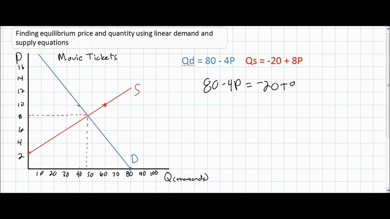
Finding Equilibrium Price and Quantity using Linear Demand and Supply Equations — This graph shows the demand and supply for movie tickets, along with their corresponding equations. The equilibrium is found where the curves intersect, which can also be solved for algebraically.

In the example above:

Demand: $Q_{d} = 80 - 4 P$
Supply: $Q_{s} = - 20 + 8 P$

Step 1: Set $Q_{d} = Q_{s}$
$80 - 4 P = - 20 + 8 P$

Step 2: Solve for P
$100 = 12 P$
$P^{*} = \frac{100}{12} \approx 8.33$
(Note: The graph shows P=8 and Q=45, which corresponds to slightly different equations, but the method is the key takeaway).

Step 3: Solve for Q
Substitute $P^{*} = 8.33$ into the demand equation:
$Q_{d} = 80 - 4 (8.33) = 80 - 33.32 = 46.68$
Or into the supply equation:
$Q_{s} = - 20 + 8 (8.33) = - 20 + 66.64 = 46.64$
(The slight difference is due to rounding P*.)

The following reading walks you through another complete algebraic example.

ECON 150: Microeconomics

This resource from a BYU Microeconomics course provides another clear, step-by-step demonstration of finding equilibrium algebraically.

Please read the section titled 'Complex Cases'. Focus on the part that starts with 'We are able to find the market equilibrium by analyzing a schedule or table, by graphing the data or algebraically.' Follow the algebraic steps shown to solve for the equilibrium quantity and then the price.

This three-pronged approach—graphical, tabular, and algebraic—gives you a robust toolkit for any equilibrium problem you might encounter.

Conclusion

In this lesson, we combined the demand and supply curves to find the heart of a market: its equilibrium. You now understand that this is more than just a point on a graph; it's the state of balance toward which a competitive market naturally gravitates.

Key Takeaways:

Market equilibrium occurs at the price where quantity demanded equals quantity supplied ( $Q_{d} = Q_{s}$ ).
You can determine the equilibrium price (P*) and quantity (Q*) in three ways:
1. Graphically: By finding the intersection point of the demand and supply curves.
2. From a schedule: By finding the price where the $Q_{d}$ and $Q_{s}$ values are identical.
3. Algebraically: By setting the demand and supply equations equal to each other and solving for price, then quantity.
Disequilibrium states of shortage ( $Q_{d} > Q_{s}$ ) and surplus ( $Q_{s} > Q_{d}$ ) create economic pressures that push the market price back toward equilibrium.

Preview of the Next Lesson:

We have now established what equilibrium is and how to find it. But what happens to this equilibrium when the underlying market conditions change? In our next lesson, we will combine the concepts from the previous lesson (curve shifters) with today's topic. We will analyze how a shift in either the demand curve, the supply curve, or both simultaneously, affects the equilibrium price and quantity.