Understanding the Fiscal Multiplier

1. The Multiplier Effect: An Intuitive Look

Imagine the government decides to spend £3 billion on building new high-speed rail lines. This money doesn't just vanish. It is paid as revenue to construction firms and as wages to workers. What happens next is the key to the multiplier effect.

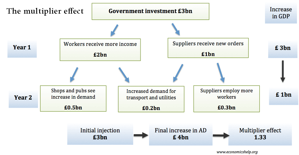
As the diagram shows, the workers and suppliers who receive the initial £3 billion will save some of it and spend the rest. Their spending—on groceries, cars, and services—becomes income for other people. This next group of people will also save some and spend the rest. This chain reaction of spending continues, with each round being smaller than the last, but adding to the total economic impact.

The fiscal multiplier is the concept that an initial change in government spending leads to a proportionally larger final change in aggregate income (and thus, GDP). The initial £3 billion in our example led to a final increase of £4 billion in GDP, implying a multiplier of 4/3 or ~1.33.

The critical factor determining the size of this effect is how much people spend out of each additional dollar of income. This brings us to the marginal propensity to consume.

2. The Marginal Propensity to Consume (MPC)

The marginal propensity to consume (MPC) is the proportion of an additional dollar of disposable income that a household spends rather than saves.

• If your MPC is 0.8, it means for every extra $100 you receive, you will spend $80 and save $20.

The MPC is the engine of the multiplier effect. A higher MPC means a larger portion of new income is re-injected into the economy at each stage, leading to a larger overall multiplier.

The following video provides a clear explanation of MPC and walks through the "follow the money" process that we just discussed.

In a simplified economy with no taxes or international trade, the multiplier formula is:

$\text{Simple Multiplier}=\frac{1}{1-\text{MPC}}$

If MPC = 0.8, the multiplier is $1/(1-0.8)=1/0.2=5$. An initial $10 billion in government spending would lead to a $50 billion increase in total income.

3. The Fiscal Multiplier in a More Realistic Economy

The simple formula is a good starting point, but for the CFA exam, you need a more realistic model that includes taxes. Taxes are a "leakage" from the circular flow of income because money paid in taxes cannot be spent by consumers.

Consumption decisions are based on disposable income, which is income after taxes. The formula for the fiscal multiplier must therefore account for the tax rate (t).

As the text explains, the formula is:

$\text{Fiscal Multiplier}=\frac{1}{1-\text{MPC}(1-t)}$

Where:

• MPC is the marginal propensity to consume.
• t is the tax rate.

The term MPC(1-t) represents the marginal propensity to consume out of total income. For every $1 of new income, t is paid in tax, leaving (1-t) as disposable income. Of that disposable income, MPC is consumed.

Notice that the tax rate t is in the denominator. This means a higher tax rate leads to a smaller fiscal multiplier, as more money leaks out of the spending stream at each round.

Practice Calculation

Let's apply this. This is a typical CFA exam-style question.

Question: An economy has a marginal propensity to consume of 0.90 and a tax rate of 30%. If the government increases spending on infrastructure by $20 billion, what is the expected total increase in aggregate demand?

Solution:

1. Calculate the multiplier:
   $\text{Multiplier}=\frac{1}{1-0.90(1-0.30)}=\frac{1}{1-0.90(0.70)}=\frac{1}{1-0.63}=\frac{1}{0.37}\approx 2.70$
2. Calculate the total increase in aggregate demand:
   $\text{Total Increase}=\text{Initial Spending}\times \text{Multiplier}=\$20\text{ billion}\times 2.70=\$54\text{ billion}$

The initial $20 billion spending program is magnified to a $54 billion impact on the economy.

4. The Balanced Budget Multiplier

What happens if the government wants to stimulate the economy without increasing its deficit? It could increase spending by $100 million and simultaneously increase taxes by $100 million. This is known as a balanced budget change. Your first thought might be that the two actions cancel each other out. However, they don't.

Let's watch the final segment of the PrepNuggets video to understand why.

Here's the logic:

• The $100 million increase in government spending (G) adds directly and fully to aggregate demand. Initial impact: +$100 million.
• The $100 million tax increase reduces household disposable income by $100 million. However, households wouldn't have spent all of that money anyway. They would have spent only MPC * $100 million. If MPC is 0.8, consumption (C) falls by only $80 million. Initial impact: -$80 million.

The net initial change in aggregate demand is +$100m - $80m = +$20 million. This positive initial change then ripples through the economy via the multiplier effect. The key takeaway is that a balanced budget fiscal expansion is still, in fact, expansionary.

5. Other Factors Affecting the Multiplier

For the CFA exam, the MPC and tax rate are the primary factors determining the multiplier's size. However, it's useful to know that other leakages can also reduce its size in the real world. The most significant is imports. When consumers receive extra income, some of it is spent on imported goods, which sends money to other countries and removes it from the domestic spending stream.

This concept is captured by the marginal propensity to import (MPI)—the fraction of additional income spent on imports.

As you can see in the formula shown, the MPI (m) is added to the denominator, reducing the multiplier's value. A higher tendency to buy foreign goods means domestic fiscal stimulus will be less effective.

Conclusion

In this lesson, we unpacked the important concept of the fiscal multiplier. We saw that fiscal policy's impact on the economy is magnified, not one-for-one.

Key Takeaways:

• The fiscal multiplier measures the final change in aggregate income that results from an initial change in government spending.
• The multiplier effect is driven by the Marginal Propensity to Consume (MPC), which is the fraction of new income that is spent.
• The exam-relevant formula for the multiplier is 1 / (1 - MPC(1 - t)).
• The size of the multiplier is positively related to the MPC and negatively related to "leakages" like the tax rate (t) and the marginal propensity to import (MPI).
• A balanced budget multiplier (where a spending increase is funded by an equal tax increase) still has a positive, expansionary effect on the economy.

Preview of the Next Lesson:

We now have the tools to understand both the direction of fiscal policy (discretionary actions and stabilizers) and the magnitude of its impact (the multiplier). In the next lesson, we will put this all together to analyze the effects of changes in government spending and taxation on aggregate demand, using the AD-AS model we developed in an earlier module.