Fiscal Policy and Aggregate Demand

1. Expansionary and Contractionary Fiscal Policy

The government has two primary levers for implementing fiscal policy: its own spending (G) and the level of taxation (T). Depending on the state of the economy, it can use these levers to either stimulate or slow down economic activity.

To understand the different policy stances, please read the following brief text.

As you just read, the two key active policy stances are:

• Expansionary Fiscal Policy: Used during a recession to boost economic activity. The government can:

  • Increase government spending (e.g., on infrastructure, defense, or social programs).
  • Decrease taxes (e.g., income tax, corporate tax), which increases households' disposable income and firms' after-tax profits.
    The goal is to increase aggregate demand.

• Contractionary Fiscal Policy: Used during an economic boom to curb inflation. The government can:

  • Decrease government spending.
  • Increase taxes.
    The goal is to decrease aggregate demand.

To see how these abstract tools translate into real-world policies, the following video provides some concrete examples.

2. The Effect of Expansionary Policy on Aggregate Demand

Let's analyze what happens when the government implements expansionary fiscal policy during a recession. The economy is operating below its potential, with high unemployment and idle resources. The government's goal is to shift the aggregate demand curve to the right.

As we learned in the last lesson, the fiscal multiplier magnifies the initial spending or tax cut. An increase in government spending (G) directly adds to aggregate demand. A cut in taxes increases disposable income, which boosts consumption (C). Both actions, amplified by the multiplier, cause the AD curve to shift to the right.

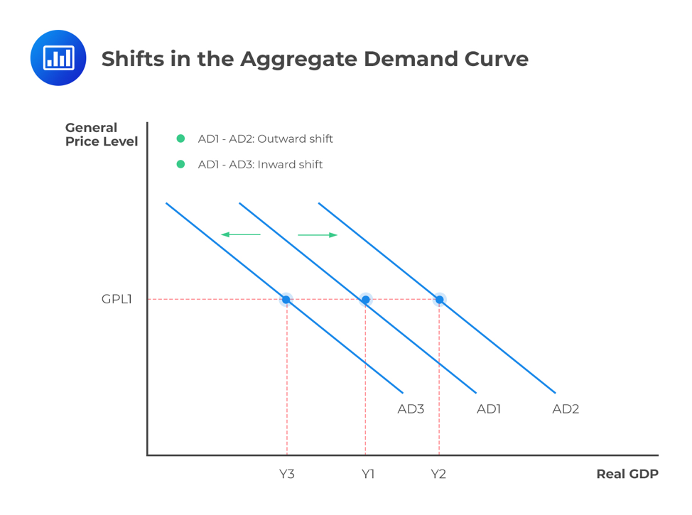
While the image above shows the shift, placing it in the full AD-AS model reveals the ultimate impact on the economy.

The key effects of an expansionary policy are:

• Real GDP increases (from Y1 to Y2), signifying economic growth.
• The price level increases (from P1 to P2), meaning there is upward pressure on inflation.
• Unemployment decreases as firms hire more workers to meet the higher demand.

The following video provides an excellent intuitive explanation for how a government spending project can ripple through the economy to achieve this result.

3. The Effect of Contractionary Policy on Aggregate Demand

Now, consider an economy that is "overheating"—producing above its long-run potential, leading to high demand-pull inflation. The government's goal is to cool things down by shifting the aggregate demand curve to the left.

To do this, it implements contractionary fiscal policy (decreasing spending or increasing taxes).

• A decrease in government spending (G) directly subtracts from aggregate demand.
• An increase in taxes reduces disposable income and corporate profits, lowering consumption (C) and investment (I).

This reduction in aggregate demand is also magnified by the multiplier effect. On the AD-AS diagram, this is represented by a leftward shift of the AD curve (e.g., from AD2 to AD1 in the graph above).

The key effects of a contractionary policy are:

• Real GDP decreases (or its growth slows), helping to bring output back towards its sustainable potential.
• The price level decreases (or its rate of increase slows), thus fighting inflation.
• Unemployment may increase as a result of the reduced economic activity.

This demonstrates the fundamental trade-off that policymakers often face between controlling inflation and maintaining low unemployment.

4. Comparing the Levers: Spending vs. Taxes

For the CFA exam, it's critical to understand that not all fiscal policy tools are created equal. Specifically, a change in government spending has a more powerful impact on aggregate demand than an equal-sized change in taxes.

Let's revisit this idea, which we touched on with the balanced budget multiplier.

Here is the core logic:

• Government Spending (G): When the government spends $100 million, the entire $100 million is a direct, first-round injection into aggregate demand.
• Tax Cut (T): When the government cuts taxes by $100 million, it increases household disposable income by that amount. However, households do not spend all of it. They spend a fraction (the MPC) and save the rest. If the MPC is 0.8, only $80 million is spent in the first round, while $20 million "leaks" into savings.

Because the initial injection from a tax cut is smaller, its final impact on aggregate demand, after the multiplier effect, will also be smaller than that of an equal-sized increase in government spending.

From the text, you saw the two simple multiplier formulas:

• Government Spending Multiplier: $\frac{1}{1-\text{MPC}}$
• Tax Multiplier: $\frac{-\text{MPC}}{1-\text{MPC}}$

Notice the tax multiplier is smaller in absolute value and negative (reflecting the inverse relationship between taxes and AD). Our more complex formula from the previous lesson, $\frac{1}{1-\text{MPC}(1-t)}$, models the effect of spending in an economy with taxes, but this comparison of the two distinct multipliers clarifies the relative power of each lever.

Conclusion

In this lesson, we analyzed how the government's fiscal tools—spending and taxation—are used to manage aggregate demand.

Key Takeaways:

• Expansionary fiscal policy (increasing spending, cutting taxes) is used in recessions. It shifts the AD curve to the right, leading to higher real GDP, a higher price level, and lower unemployment.
• Contractionary fiscal policy (decreasing spending, raising taxes) is used to fight inflation. It shifts the AD curve to the left, leading to lower real GDP (or slower growth), a lower price level, and potentially higher unemployment.
• A dollar of government spending has a more powerful impact on aggregate demand than a dollar of tax cuts, because the full amount of spending is injected directly into the economy, while a portion of a tax cut is saved.

Preview of the Next Lesson:

When the government uses expansionary policy, it often spends more than it collects in tax revenue, creating a budget deficit. When it uses contractionary policy, it may collect more than it spends, creating a budget surplus. In our next lesson, we will explore the crucial relationship between these annual deficits and surpluses and the long-term accumulation of national debt.