Hello. Last lesson separated what an excluded pathway does during the intact computation from what it can do after the candidate circuit is removed. This lesson examines a related trap: an intervention can make a model use a pathway that was inactive on every unmodified input. You will calculate the effect in a three-unit network, reproduce it with a PyTorch hook, and use the result to sharpen what a successful activation patch does—and does not—establish.
A successful patch is not always a faithful explanation
An activation patch replaces part of a destination run’s hidden state with information from a source run. If the destination output changes to match the source output, the patched direction has interventional control over that output. A stronger claim would be that the model normally uses that direction to carry the relevant information. The two claims can come apart.
One way this happens is when a direction combines two otherwise unremarkable pieces:
- A disconnected component varies with the input, but its variation cannot reach the output.
- A dormant component could affect the output if changed, but never changes across the ordinary inputs being studied.
A patch along their mixture can take an input-dependent difference from the disconnected component and write part of it into the dormant component. The output then changes through a route the unmodified model did not use.
Read the paper’s explanation of how a successful subspace patch can combine input information with an unused route to the output.
In Section 3.2, “Intuition for the Illusion,” begin at “The crux of the illusion is that” and read the construction through the discussion following Equation (3). Focus on why patching either component alone fails while patching their mixture works. You can skim the algebraic formatting on a first pass; the calculation below makes it concrete. Stop before the paragraph beginning “We make the concepts,” which turns to formalization and an optimality result.
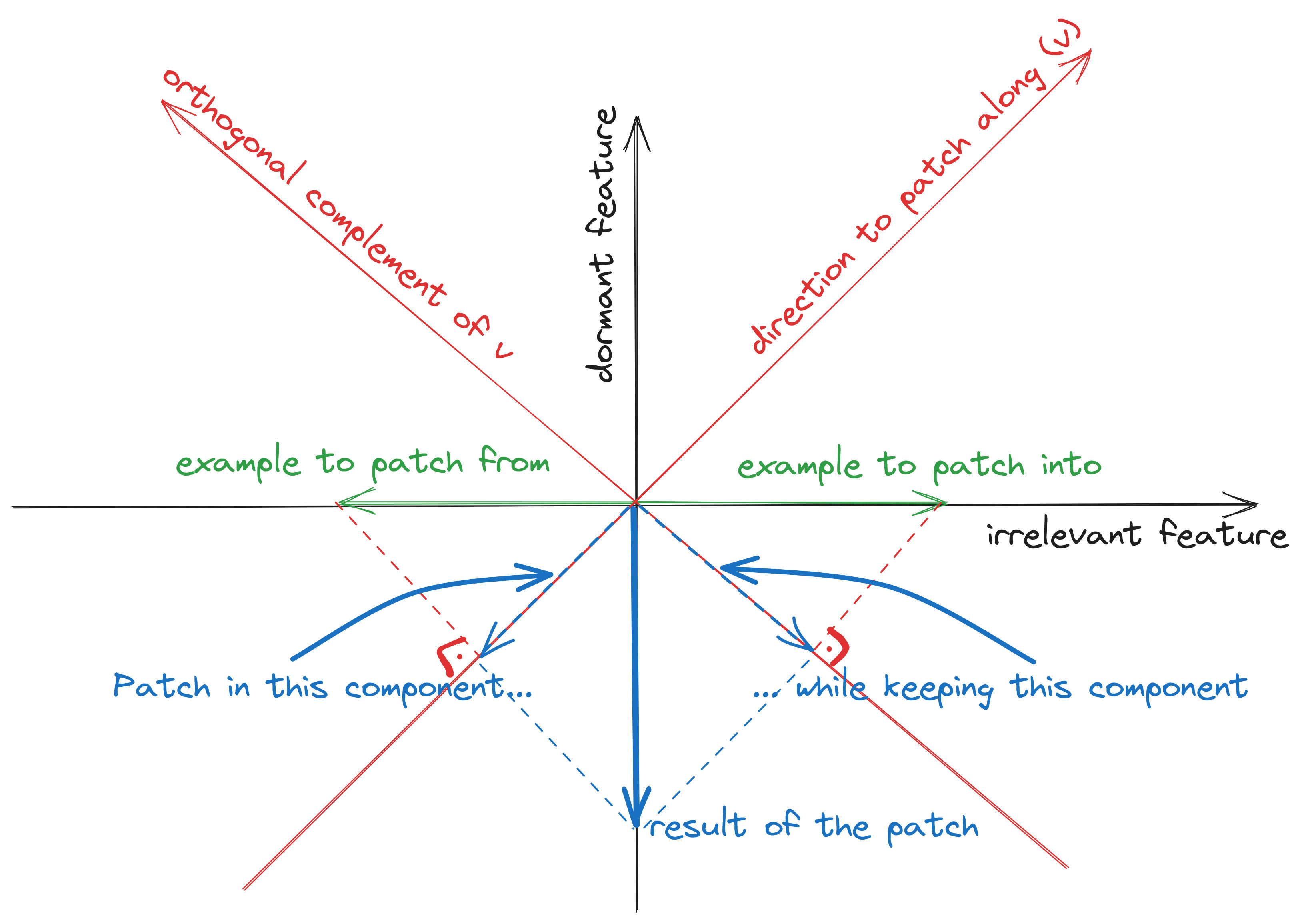
The sketch is an intuition, not evidence about a particular model. To see exactly which route is used, we need to inspect both the ordinary hidden states and the patched one.
A three-unit network with two explanations for the same patch result
Consider a deliberately simple network with scalar input , hidden state , and scalar output :
On an ordinary forward pass, the input reaches the output through . The other coordinates have different properties:
- tracks the input, but its output weight is zero.
- for every ordinary input, but its output weight is two.
- both tracks the input and contributes to the output.
Now use and . Their hidden states are and , and their ordinary outputs are and .
For a unit direction , a one-dimensional source-to-base patch replaces the base state’s projection onto with the source state’s projection:
Take the mixed direction
The source–base difference is , so its projection onto is . The patch therefore adds to the base state:
The intervention perfectly transfers the source output, yet —the coordinate that carried the input to the output in both ordinary runs—still has its base value of . The change in output comes entirely from , which was zero in both ordinary runs. Indeed, is not a hidden state this network produces from any unmodified scalar input: its ordinary states must have and .
Read the paper’s original version of this network to connect the calculated patch to its distinction between disconnected, dormant, and faithful directions.
In Section 3.3, “The Illusion in a Toy Model,” start at “With these concepts in mind” and read the toy construction, continuing through the final equation at the end of the subsection. Compare the paper’s three coordinate descriptions with the ordinary state (x,0,x), then check which coordinate produces the final output after the mixed-direction patch. The following Section 3.4 begins a different topic and is not needed here.
For arbitrary source and base inputs, the same calculation yields
Thus this is not a numerical coincidence of and . The patch succeeds for any pair, despite leaving the ordinary output-carrying coordinate at its base value.
Reproduce the effect with an activation hook
The following self-contained PyTorch model exposes its hidden state as an nn.Identity module so a forward hook can modify precisely that state. It caches the source activation, then compares patches along the disconnected coordinate, dormant coordinate, faithful coordinate, and mixed direction.
import torch
from torch import nn

class ToyNetwork(nn.Module):
    def __init__(self):
        super().__init__()
        self.hidden = nn.Identity()
        self.register_buffer("w1", torch.tensor([1.0, 0.0, 1.0]))
        self.register_buffer("w2", torch.tensor([0.0, 2.0, 1.0]))

    def forward(self, x):
        h = self.hidden(x * self.w1)
        return torch.dot(h, self.w2)

model = ToyNetwork()
x_source = torch.tensor(3.0)
x_base = torch.tensor(1.0)

cache = {}

def save_source(_module, _inputs, h):
    cache["source"] = h.detach().clone()

handle = model.hidden.register_forward_hook(save_source)
source_output = model(x_source).item()
handle.remove()
base_output = model(x_base).item()

def run_patch(direction):
    direction = direction / direction.norm()
    seen = {}

    def replace_projection(_module, _inputs, h):
        source = cache["source"]
        patched = h + torch.dot(source - h, direction) * direction
        seen["hidden"] = patched.detach().clone()
        return patched

    handle = model.hidden.register_forward_hook(replace_projection)
    try:
        output = model(x_base).item()
    finally:
        handle.remove()
    return seen["hidden"], output

directions = {
    "disconnected h1": torch.tensor([1.0, 0.0, 0.0]),
    "dormant h2": torch.tensor([0.0, 1.0, 0.0]),
    "faithful h3": torch.tensor([0.0, 0.0, 1.0]),
    "mixed h1+h2": torch.tensor([1.0, 1.0, 0.0]),
}

print("ordinary base/source outputs:", base_output, source_output)
for label, direction in directions.items():
    hidden, output = run_patch(direction)
    print(label, hidden.tolist(), output)
The expected results are:
| Patched direction | Resulting hidden state | Output |
|---|---|---|
| alone | ||
| alone | ||
| alone | ||
| Mixed |
The two successful patches have different mechanisms. Patching transfers a value along the route used in ordinary computation. Patching the mixture uses the difference stored in to create a new, output-changing value in . Patching alone changes something the readout ignores; patching alone transfers zero from the source, so it changes nothing.
The hook makes the intervention a genuine causal manipulation of this toy model. It does not make the mixed direction a faithful account of the model’s unmodified computation. Successful control and faithful attribution are separate findings.
Diagnose the pathway, not just the output change
In this toy network, three checks expose the illusion.
First, inspect ordinary activations and contributions over the input distribution. and its contribution are always zero, while varies with and contributes . A derivative alone would miss this distinction: the output is sensitive to a hypothetical change in , even though the model never makes such a change on an ordinary run.
Second, inspect the post-patch state and route. The mixed patch makes , contributing two output units, while stays at its base value. This identifies how the patched run succeeded, rather than inferring a route from the final output alone.
Third, compare component-only and faithful-direction patches. Neither nor alone transfers the output; does. The mixed direction succeeds by combining the input variation of one component with the downstream influence of another. Reversing the source and base also changes the output in the opposite direction, but that additional patching result still does not make the dormant route active in ordinary computation.
The paper reports a related analysis in a transformer: it compares a successful subspace intervention with interventions on the whole MLP activation and on components of the direction that differ in their ability to distinguish examples or affect downstream computation. Its empirical setting is more complex than this exact toy construction, so read those comparisons as a method of investigating the suspected route, not as a claim that every effective patch is illusory.
See how the paper tests for a similar mismatch between an effective patch and an MLP’s ordinary contribution in a transformer.
In Section 4.4, “Results: Demonstrating the Illusion for the MLP Direction,” inspect the table at the start, then read the comparisons from “Methodology and interventions considered” through the paragraph under “Patching ... activates a dormant pathway through the MLP.” Focus on why the authors compare a direction patch with a full-component patch and with its nullspace and rowspace components. Stop before “Further validations of the illusion”; the remaining subsections are not required for this lesson.
For a real model, “inactive” is usually an empirical, distribution-relative judgment rather than the exact zero proved here. A robust claim needs ordinary-run measurements on held-out inputs, targeted comparisons of candidate routes, and attention to the replacement policy and behavior metric. An unusual patched state is a reason to investigate; being off the ordinary-state manifold is not, by itself, a proof that an intervention is uninformative.
Conclusion
The toy network computes through on every unmodified run. Nevertheless, patching a mixture of input-tracking and dormant transfers the source output perfectly by activating . A patch can establish that a model can use a pathway under intervention without establishing that it does use that pathway ordinarily. Inspecting natural activations, patched states, and downstream contributions makes that distinction testable.
This completes the circuits module. Next, the course turns to sparse autoencoders, beginning with why a network might represent more sparse features than it has activation dimensions—a motivation for searching beyond individual neurons.