Welcome to the module on sparse autoencoders. Its starting point is a representational puzzle: a model can usefully track more features than an activation vector has dimensions. Before studying methods that try to separate those features, we need a concrete account of how they can fit together in the first place.
This lesson builds that account with a small reconstruction model. You will see what “more features than dimensions” means mathematically, why sparse features make the arrangement useful despite interference, and what the toy model does—and does not—establish about real networks.
Features are not necessarily coordinates
Suppose an activation vector has two coordinates. It has only two mutually orthogonal axes, but a feature need not occupy an axis. It can contribute a vector pointing in any direction in the plane. If several features are present, their contributions can add:
Here is the strength of feature , is its direction, and is the resulting activation. The map from feature strengths to activations is linear; the features themselves could be complicated properties of an input.
A coordinate of may therefore respond to several features. Conversely, one feature may change both coordinates. This is why finding a responsive neuron is not, by itself, the same as identifying a feature.
Read the definitions in Toy Models of Superposition by Elhage and colleagues to establish what the authors mean by feature directions and superposition.
In “Definitions and Motivation: Features, Directions, and Superposition,” read “Features as Directions” from linear representations. Then read “The Superposition Hypothesis” from the hypothesis. Focus on the distinction between a feature direction and a coordinate, and on the cost of making feature directions non-orthogonal.
A useful way to inspect that cost is to read feature back out by taking a dot product with its direction. Before any threshold or bias, the readout is
The first term is the desired signal. The remaining terms are interference from other active features. Orthogonal directions make those terms zero; using more nonzero directions than dimensions means they cannot all be orthogonal. Superposition is the choice to represent extra features anyway, accepting some interference rather than omitting those features.
Two features in one dimension
We can make the tradeoff exact without training a network. Let and be nonnegative features, each either 0 or 1. Give them opposite directions in a one-dimensional hidden space:
Decode with the transpose of and a ReLU:
When only is present, and the decoder returns . When only is present, and it returns . One activation dimension has successfully represented two distinguishable features. The sign distinguishes them, while ReLU clips the negative readout for the absent feature.
The arrangement fails when both features are present. Then , exactly as when neither is present, so the decoder cannot recover the pair. This is a collision, not a violation of the dimensional limit: the one-dimensional representation never retained enough information to reconstruct every possible combination.
Sparsity can make that loss worthwhile. Suppose and activate independently, each with probability , and measure error by squared reconstruction error summed over both features. The opposite-direction scheme errs only when both are present. Its expected loss is
A different scheme could represent perfectly and ignore . It errs whenever is present, giving
At , those losses are and , respectively. At , they are and . These comparisons concern two specified encoding schemes, not a claimed universal optimum. They expose the central bargain: if features are rarely active together, paying for occasional collisions can be cheaper than never representing one of them.
From the construction to a trained toy model
The research toy model extends this idea to multiple synthetic features. It compresses an input into a smaller hidden vector , then attempts to reconstruct :
Each column is the hidden-space direction assigned to input feature . The model is trained to reduce expected reconstruction error, with larger penalties for mistakes on more important features. Its synthetic inputs also let the researchers control sparsity: how often each feature is absent. Unlike our binary construction, a feature that is present can have a value between 0 and 1.
Continue with the paper’s experimental setup and basic results. The value of this reading is that its feature directions are learned, rather than selected by hand as in our one-dimensional construction.
Under “Demonstrating Superposition,” read “Experiment Setup”: in “The Feature Vector (x),” begin at the synthetic features; in “The Model (x to x'),” read from the two models; and read the short “The Loss” subsection. Then read “Basic Results” from the trained results, including its figures. Stop before “Mathematical Understanding.” Track which feature vectors have appreciable length, and whether those vectors are orthogonal.
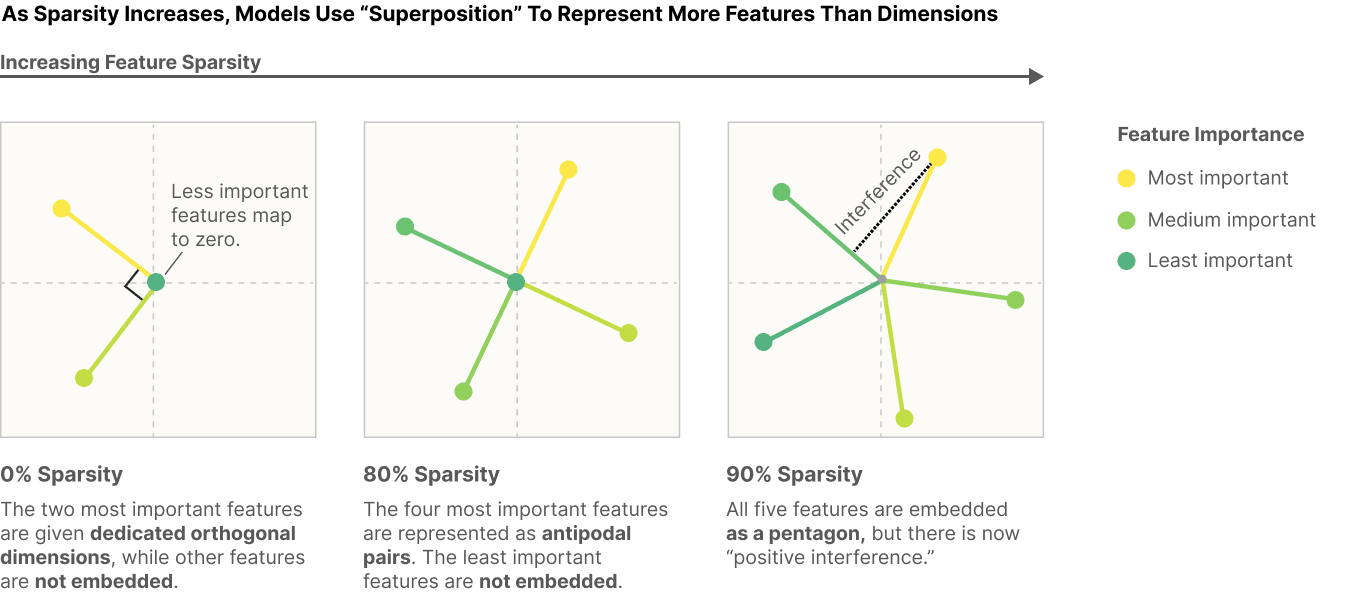
The important observation is not merely that a diagram contains many arrows. In the paper’s trained ReLU-output models, increasing feature sparsity changes the learned solution: directions for additional features acquire appreciable length and share the available dimensions. When features are dense, the model instead tends to reserve relatively clean directions for important features and leave others unrepresented. The linear-output comparison helps isolate the role of the output nonlinearity in this particular setup.
With five features in two dimensions, opposite pairs are no longer the whole story. The model can spread directions around the plane. A direction with a positive dot product against another can produce a false readout even when only one of those features is present. Negative overlaps can be clipped by ReLU; a learned negative bias can also suppress small positive false readouts, although filtering too aggressively risks suppressing genuine weak signals. Thus “features collide only when both activate” is an exact description of our simple opposite-direction construction, not a general rule for every superposed arrangement.
Superposition: More Features Than Neurons
Watch “Superposition: More Features Than Neurons” from DataMListic for a visual account of a trained five-feature, two-dimensional example. Use its plots to connect vector length and angle to the reconstruction tradeoff, rather than treating a tidy shape alone as proof of what a feature means.
In the setup, identify the five input features, two-dimensional bottleneck, and weighted reconstruction objective. Compare dense training with sparse training: note which directions collapse toward zero and which remain represented. Finish with the neuron view, which shows why an individual coordinate can mix contributions from several feature directions.
What this explains—and what it leaves open
In the toy model, the input features are specified in advance. We know which synthetic property each input coordinate stands for, can inspect its learned direction, and can measure reconstruction error. That makes it a clean demonstration that a trained nonlinear network can benefit from representing more sparse features than hidden dimensions. It also explains one route to a polysemantic neuron: a single activation coordinate can receive contributions from several off-axis feature directions.
A real model presents a harder problem. Its candidate features are not supplied as labeled input coordinates, and an appealing collection of activation vectors does not establish their meanings or whether the model uses them for a claimed behavior. The toy result motivates searching for features that do not align with individual neurons; it does not validate any particular semantic label assigned to a real activation. Later lessons will separate feature discovery from tests of downstream behavioral effect.
Key takeaways
Superposition stores more features than dimensions by assigning features non-orthogonal directions. It works imperfectly: overlapping directions create interference, but sparsity and a nonlinear readout can make the resulting expected error preferable to dropping useful features. The one-dimensional example shows the bargain exactly; the trained toy model shows how related arrangements can emerge under a reconstruction objective.
Next, the module turns to sparse autoencoders, which attempt to recover a more interpretable set of features from activations that may contain such mixtures.