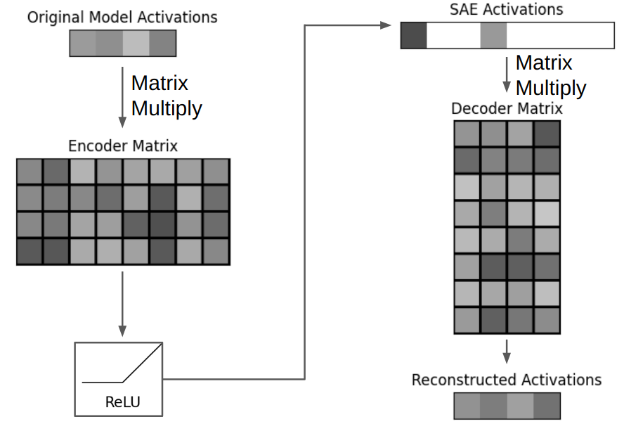
Welcome back. The previous lesson showed why sparse features might be mixed across fewer activation dimensions than there are features. A sparse autoencoder (SAE) tackles the reverse problem: given activation vectors from a fixed model location, learn a wider set of components that can reconstruct those vectors while using only a few components at a time.
This lesson takes that idea through a complete small PyTorch fit. The activations will be cached before SAE training, so the distinction stays clear: the SAE learns from the model’s activations; it does not train the original model.
What the SAE is trained to do
For an activation vector of dimension , an SAE produces a vector of latent activations, usually with :
The encoder finds candidate latent activations; the decoder uses them to reconstruct the original vector. The decoder’s column for latent is the contribution that one unit of makes to . These learned latents are not the known input features in last lesson’s toy model: their identities are not supplied to the SAE.
Watch the construction in Welch Labs’ The Dark Matter of AI. Focus on the choice of one model location and on why reconstruction must be paired with pressure to use few latent entries. Treat the video’s proposed “concepts” as candidate interpretations, not labels established by the training procedure.
The Dark Matter of AI [Mechanistic Interpretability]
Watch the SAE construction in The Dark Matter of AI by Welch Labs for a visual account of the encoder, sparse intermediate representation, and decoder.
Watch the SAE construction. The explanation starts by selecting activations at a target location, then builds the wider encoded vector and its reconstruction. Focus on which quantities are learned by the SAE and which activations come from the original model.
ReLU makes each nonnegative, but it does not, by itself, guarantee that few entries are nonzero. A simple training loss adds an L1 penalty on the latent activations, not on the weights:
Here is batch size, and sets the reconstruction–sparsity trade-off. Since ReLU makes nonnegative, its L1 norm is simply the sum of its entries. A large makes activity expensive but may discard information; a small one may produce excellent reconstruction with little sparsity. Neither term rewards semantic interpretability directly.
Cache first, then fit
An SAE is trained on activations collected at a specified location in a frozen source model. If you use a hook on a transformer, decide which layer output and token positions count as examples, run inputs through the model without gradients, and store detached activation vectors of shape [number_of_examples, D]. Keep validation inputs separate. For text, splitting by document or source example before collecting token activations avoids putting closely related tokens on both sides of the split.
The following scaffold uses a fixed synthetic source instead of requiring a transformer download. It mixes twelve occasionally active source features into eight-dimensional vectors and caches the resulting vectors once. The SAE receives only those eight-dimensional vectors, not the source-feature values or mixing directions. Thus the fit has the same data interface as one trained on hooked activations, while remaining runnable on a CPU.
Before running it, read Adam Karvonen’s An Intuitive Explanation of Sparse Autoencoders for LLM Interpretability for its compact encode/decode scaffold and loss. Our implementation makes one scaling choice explicit: both loss terms are averaged per example. That keeps the meaning of consistent when batch size changes; the reference loss averages reconstruction error but sums latent activity over the whole batch.
An Intuitive Explanation of Sparse Autoencoders for LLM Interpretability | Adam Karvonen
Read Adam Karvonen’s account for the data-collection setup, the reference PyTorch SAE class, and the reconstruction-plus-L1 objective. Compare its shapes and loss reductions with the scaffold below.
In “Sparse Autoencoder Explanation,” under “How Sparse Autoencoders Work,” scroll past the architecture diagram and large-model dimension example. Begin at “We train individual SAEs on only one location in the model.” Read the data setup. Continue through the paragraph introducing the reference PyTorch implementation and its SparseAutoEncoder class, ending at the class’s return reconstructed_model_activations_D, encoded_representation_F line. Immediately below, read the loss explanation and the calculate_loss code that follows, ending at return loss. Notice especially what is penalized and how each term is reduced across the batch.
The cache can now be created and the SAE fitted in one script. The decoder columns are kept at unit norm. Without a norm constraint, the encoder could shrink while the decoder enlarges its columns, retaining much the same reconstruction but making the L1 penalty artificially cheap.
import torch
from torch import nn
from torch.nn import functional as F
from torch.utils.data import DataLoader, TensorDataset

torch.manual_seed(2)
generator = torch.Generator().manual_seed(71)

activation_dim = 8
source_feature_count = 12
dictionary_size = 24
l1_coefficient = 0.02

# Fixed source: generate activations once, then train only on the cache.
source_directions = F.normalize(
    torch.randn(source_feature_count, activation_dim, generator=generator),
    dim=1,
)

@torch.no_grad()
def collect_activations(n):
    present = (
        torch.rand(n, source_feature_count, generator=generator) < 0.10
    )
    strengths = (
        0.6 + 0.8 * torch.rand(n, source_feature_count, generator=generator)
    )
    source_values = present.float() * strengths
    noise = 0.01 * torch.randn(n, activation_dim, generator=generator)
    return source_values @ source_directions + noise

torch.save(
    {
        "train": collect_activations(4096),
        "valid": collect_activations(1024),
    },
    "toy_activations.pt",
)
cache = torch.load(
    "toy_activations.pt", map_location="cpu", weights_only=True
)
train_x, valid_x = cache["train"], cache["valid"]
assert train_x.shape == (4096, activation_dim)
assert valid_x.shape == (1024, activation_dim)


class SparseAutoencoder(nn.Module):
    def __init__(self, input_dim, latent_dim):
        super().__init__()
        self.encoder = nn.Linear(input_dim, latent_dim)
        self.decoder = nn.Linear(latent_dim, input_dim)
        self.constrain_decoder()

    @torch.no_grad()
    def constrain_decoder(self):
        # nn.Linear stores decoder weights as [input_dim, latent_dim].
        self.decoder.weight.copy_(
            F.normalize(self.decoder.weight, dim=0)
        )

    def forward(self, x):
        z = F.relu(self.encoder(x))
        reconstruction = self.decoder(z)
        return reconstruction, z


sae = SparseAutoencoder(activation_dim, dictionary_size)
optimizer = torch.optim.Adam(sae.parameters(), lr=1e-3)
loader = DataLoader(
    TensorDataset(train_x), batch_size=256, shuffle=True
)

@torch.no_grad()
def report(model, x):
    model.eval()
    reconstruction, z = model(x)
    error_per_example = (reconstruction - x).square().sum(dim=1)
    activity_per_latent = (z > 1e-6).float().mean(dim=0)
    return {
        "reconstruction_error": error_per_example.mean().item(),
        "active_latents_per_example":
            (z > 1e-6).sum(dim=1).float().mean().item(),
        "never_active_latents": (activity_per_latent == 0).sum().item(),
    }

for epoch in range(1, 31):
    sae.train()
    for (x,) in loader:
        reconstruction, z = sae(x)
        reconstruction_loss = (
            (reconstruction - x).square().sum(dim=1).mean()
        )
        sparsity_loss = l1_coefficient * z.sum(dim=1).mean()
        loss = reconstruction_loss + sparsity_loss

        optimizer.zero_grad()
        loss.backward()
        optimizer.step()
        sae.constrain_decoder()

    if epoch in (1, 10, 20, 30):
        print(epoch, report(sae, valid_x))

# A constant reconstruction using only the training-set mean.
mean_reconstruction = train_x.mean(dim=0)
baseline_error = (
    (valid_x - mean_reconstruction).square().sum(dim=1).mean()
)
print("mean-only validation error:", baseline_error.item())
print("final validation metrics:", report(sae, valid_x))
This is a fit, not a test of feature meaning. The optimizer updates the encoder and decoder to reduce the stated loss. It never sees source_values or source_directions; those variables exist solely to generate a reproducible cache. With real hooked activations, train_x and valid_x would be replaced by your detached tensors, while the SAE and training loop could remain substantially the same.
Reading the fit without overclaiming
The reported reconstruction error is the mean sum of squared errors across activation dimensions per example—the same reconstruction quantity used in training. Compare its validation value with the mean-only baseline. A lower value establishes that the SAE reconstructs held-out vectors better than that simple constant predictor; it does not establish that reconstruction is accurate enough for a downstream use.
active_latents_per_example is an empirical L0 count: how many entries of exceed a small threshold for an average validation example. It is useful to inspect alongside reconstruction error, but it is not the L1 quantity being optimized. For example, fewer nonzero entries with very large values can have a different L1 cost from more entries with small values. never_active_latents flags units that did not activate anywhere in this validation cache; it is not proof that they would never activate on other data.
Several comparisons keep the fit interpretable:
- If reconstruction improves while nearly all 24 latents fire on each example, the SAE has not achieved the intended sparse code.
- If very few latents fire but reconstruction remains poor, sparsity may be too expensive relative to reconstruction at this .
- If training error is much better than validation error, inspect how the cache was sampled and whether its validation distribution matches the intended use.
The numerical balance depends on activation scale, dictionary size, data distribution, and decoder constraints. In particular, changing the loss from a sum of squared errors across dimensions to a mean across dimensions changes the effective strength of the same . Keep the loss definition fixed when comparing runs.
Most importantly, a low-error sparse decomposition need not recover the twelve source features one-for-one. Multiple dictionaries can reconstruct similar data; noise and finite samples also affect what is learned. In a real network, there are no supplied source-feature labels to settle that question. Inspecting which inputs activate a latent and testing what changing it does require separate work.
Key takeaways
You have fitted an overcomplete SAE to cached, held-out-evaluable activations using a per-example reconstruction error plus an L1 penalty on encoded activity. The encoder and decoder learn a sparse reconstruction of vectors from one fixed source location; decoder norm control prevents an easy scaling workaround. Validation reconstruction and activity counts show whether that objective was achieved, not whether the latents are meaningful or causally important.
The next lesson asks a different question: if SAE reconstructions replace the original activations inside a model, how much do they distort its downstream behavior?