Last lesson fitted an SAE to cached activations and measured how accurately and sparsely it reconstructed held-out vectors. That leaves a consequential gap: a small reconstruction error does not tell you whether the model can still use the reconstructed activation. The omitted information might lie in directions that matter greatly to its predictions.
Here you will put the reconstruction back at the activation site, run the frozen model’s remaining computation, and measure the change in output behavior. The distinction is central to your broader goal: reconstruction fidelity describes the SAE’s approximation; downstream fidelity tests what happens when the model must rely on it.
What to measure after a reconstruction splice
Let be the original activation at a specified model site and its reconstruction. Compare two forward passes on the same held-out inputs: one leaves untouched, while the other substitutes at that site. Keep the model, prompts, prediction positions, and all other conditions fixed.
For a language model, two complementary measurements are:
where cross-entropy (CE) uses the actual held-out next tokens as targets, and
which compares the model’s full next-token distributions. A positive means the substitution worsened average prediction of the observed tokens. KL is nonnegative and measures departure from the clean model, whether or not that departure improves CE on a particular sample. Report which distribution comes first: KL is asymmetric.
Read “4.1 Downstream loss” in Scaling and evaluating sparse autoencoders. The authors explain why activation-space error may miss behaviorally important information, use both KL and cross-entropy, and caution against an apparently impressive normalization.
Scaling and evaluating sparse autoencoders
Read the paper’s “4.1 Downstream loss” subsection to connect reconstruction quality with model-output measurements.
Start at the paragraph beginning “An autoencoder with non-zero reconstruction error may not succeed.” Read through the baseline discussion. Focus on what is replaced during the forward pass, why the authors report a change in cross-entropy, and why zero-ablation can make “loss recovered” look generous.
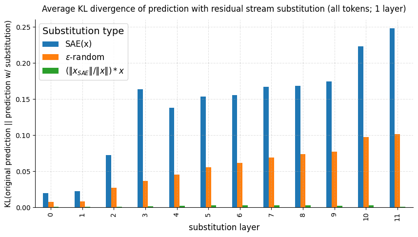
Neither metric follows automatically from last lesson’s mean squared reconstruction error. Squared error weights differences by their size in activation space; the downstream network need not weight all activation directions equally. Nor does a favorable average KL rule out large damage on a small, important subset of inputs. The bar chart below illustrates that substitution effects can also depend strongly on the layer chosen. Its three substitution types are not, by themselves, a controlled comparison of equal-error perturbations; read it as a reason to specify the intervention and measure its output, not as a verdict on any particular SAE.
A held-out measurement with a PyTorch hook
The previous lesson’s synthetic source produced activation vectors but did not include a downstream model. A cache alone cannot establish behavioral distortion: something must consume the activation after the splice. The following experiment adds a small frozen readout after the same eight-dimensional activation site. It is a deliberately limited stand-in for the remaining blocks and output head of a language model.
Run this after the previous lesson’s script, with sae, train_x, activation_dim, and collect_activations still available. It draws fresh test activations, which were not used to fit the SAE. Synthetic target labels come from a separate fixed rule; the frozen readout approximates that rule. Thus CE refers to labels not supplied to the SAE, while KL refers to the readout’s clean predictions.
import torch
from torch import nn
from torch.nn import functional as F

rng = torch.Generator().manual_seed(109)
test_x = collect_activations(4096)  # fresh inputs, not SAE training data

# Synthetic target rule and a distinct, frozen downstream readout.
n_classes = 5
target_w = 2.0 * torch.randn(
    activation_dim, n_classes, generator=rng
)
readout_w = target_w + 0.12 * torch.randn(
    activation_dim, n_classes, generator=rng
)
targets = (test_x @ target_w).argmax(dim=-1)


class ToyContinuation(nn.Module):
    def __init__(self, dim, classes):
        super().__init__()
        self.site = nn.Identity()  # explicit, hookable activation site
        self.readout = nn.Linear(dim, classes, bias=False)

    def forward(self, x):
        return self.readout(self.site(x))


continuation = ToyContinuation(activation_dim, n_classes)
with torch.no_grad():
    continuation.readout.weight.copy_(readout_w.T)
continuation.eval()
sae.eval()


def logits_with_splice(x, replacement=None):
    """Run the frozen continuation, optionally replacing its site output."""
    if replacement is None:
        return continuation(x)

    def hook(_module, _inputs, output):
        substituted = replacement(output)
        assert substituted.shape == output.shape
        return substituted

    handle = continuation.site.register_forward_hook(hook)
    try:
        return continuation(x)
    finally:
        handle.remove()


# A baseline mean must come from training data, not the test set.
train_mean = train_x.mean(dim=0, keepdim=True)

with torch.no_grad():
    clean = logits_with_splice(test_x)
    identity = logits_with_splice(
        test_x, lambda x: x.clone()
    )
    sae_logits = logits_with_splice(
        test_x, lambda x: sae(x)[0]
    )
    zero = logits_with_splice(
        test_x, lambda x: torch.zeros_like(x)
    )
    mean = logits_with_splice(
        test_x, lambda x: train_mean.expand_as(x)
    )

    # Control: random error with the SAE's error norm for each example.
    reconstruction, _ = sae(test_x)
    error_norm = (reconstruction - test_x).norm(
        dim=-1, keepdim=True
    )
    random_direction = F.normalize(
        torch.randn(test_x.shape, generator=rng), dim=-1
    )
    matched_noise = logits_with_splice(
        test_x,
        lambda x: x + random_direction * error_norm,
    )

    conditions = {
        "clean": clean,
        "identity": identity,
        "SAE": sae_logits,
        "zero": zero,
        "train mean": mean,
        "matched-norm noise": matched_noise,
    }
    clean_probs = F.softmax(clean.float(), dim=-1)
    clean_ce = F.cross_entropy(clean.float(), targets).item()

    results = {}
    for name, logits in conditions.items():
        logits = logits.float()
        ce = F.cross_entropy(logits, targets).item()
        # F.kl_div(input_log_q, target_p) computes KL(p || q).
        kl = F.kl_div(
            F.log_softmax(logits, dim=-1),
            clean_probs,
            reduction="batchmean",
        ).item()
        results[name] = ce
        print(
            f"{name:19s} CE={ce:.4f}  "
            f"delta CE={ce - clean_ce:+.4f}  "
            f"KL(clean || condition)={kl:.4f}"
        )

    print(
        "largest identity-logit difference:",
        (identity - clean).abs().max().item(),
    )
The hook returns a new activation at the site before the readout consumes it. It is removed in finally, so one condition cannot silently alter the next. The identity condition exercises the same hook path while writing back unchanged values; its logits should match clean up to numerical precision. If they do not, resolve the measurement setup before interpreting the SAE result.
The SAE condition replaces the whole activation with . It does not preserve the original reconstruction residual . That matters: retaining the residual would restore information the SAE failed to encode and answer a different question. A later lesson will use residual preservation when isolating the effect of one latent.
The zero and training-mean conditions supply reference points for how disruptive a much cruder replacement is. The matched-norm-noise condition asks a narrower question: does the SAE’s error direction cost more than a random direction with the same error magnitude on each test example? It is a control, not a substitute for the SAE measurement.
Interpreting the numbers without hiding the damage
Begin with the absolute results: clean CE, SAE CE, their difference, and clean-to-SAE KL, all on the same held-out examples. Check the identity result. Then inspect the baselines. A common supplementary statistic is loss recovered relative to a specified ablation:
It equals one when the SAE matches clean CE and zero when it matches the chosen baseline CE, provided the baseline is meaningfully worse than clean. It is not an absolute measure of negligible distortion. If zeroing the site is catastrophic, an SAE can recover a high fraction of that enormous gap while still adding a consequential amount of CE. A training-mean baseline may give a less extreme comparison; always name the baseline and report the unnormalized difference as well. If a baseline’s CE is close to clean CE, the fraction is unstable and should not be emphasized.
The Evaluating SAEs tutorial offers a useful diagnostic example. Read its downstream-loss setup, then follow how an unexpectedly large loss is traced to a token position the SAE was not trained to reconstruct. Its later matched-norm control illustrates why equal-sized activation errors need not have equal behavioral costs.
Read the nnsight tutorial’s “Step 4: Downstream loss recovered,” “Step 5: The diagnosis,” and “Step 6: A control that reframes FVU.” It is a practical example of measuring and debugging a reconstruction splice in a language model.
In Step 4, begin at “FVU says the SAE discards 20% of the variance” and read through the loss-recovered definition. Skim the condition code for which positions each replacement affects. In Step 5, start “Work from the cheapest suspect outwards” and read the identity and position diagnosis; focus on why leaving the first token untouched changes the conclusion. In Step 6, read from “We now have a clean set of numbers” through the matched-error setup, then read its interpretation.
That example exposes a general failure mode. “Replace the activations” is incomplete as an experimental specification. You must say which layer and site, which token positions, and which population of inputs the SAE was trained on. If special or padding positions were excluded from SAE training, splicing their reconstructions into a language model can badly distort later predictions. Keep the intervention mask identical across SAE and baseline conditions, and inspect per-position loss if the aggregate is surprising.
Our toy continuation has only one activation vector per example, so it cannot exhibit attention-mediated contamination across positions. In a transformer, the corresponding procedure uses a hook at the SAE’s exact training site, substitutes reconstructions only at the intended positions, and computes CE from the model’s final logits with the usual next-token alignment. Intermediate head outputs are not necessarily final logits if the architecture applies further transformations. Report how many held-out sequences and predicted tokens contributed to each average.
Finally, interpret a good result narrowly. Small SAE-induced KL and show that the complete reconstruction supports much of the measured downstream behavior on the tested distribution. They do not establish that any individual latent has a particular meaning, that the model normally computes with those latents, or that rare target behaviors are preserved. Those claims require their own held-out and causal tests.
Key takeaways
To measure downstream distortion, splice an SAE reconstruction into a frozen model at its matched activation site and compare outputs on identical held-out inputs. Report delta CE and/or clean-to-intervened KL, verify an identity splice, and use explicitly named zero, mean, or matched-error controls to put the result in context. Activation reconstruction error alone cannot tell you what information the downstream model misses; a high loss-recovered fraction alone can conceal a substantial absolute loss.
The next lesson turns from the whole dictionary to an individual latent: whether a proposed semantic description survives held-out positive examples, counterexamples, and nearby concepts.