Introduction
In our last lesson, we explored the Mean Value Theorem, which provides a profound connection between the average rate of change of a function over an interval and its instantaneous rate of change at a specific point. We concluded by noting that this theorem has powerful consequences for understanding a function's behavior.
Today, we will investigate the first of these major consequences. We will learn how to use the sign of the first derivative () to determine precisely where a function is increasing (going "uphill") or decreasing (going "downhill"). This will lead us directly to a systematic method for finding the local peaks and valleys of a function's graph, known as local extrema. This powerful technique, the First Derivative Test, is a cornerstone of calculus and a fundamental tool for sketching graphs and solving optimization problems. This lesson corresponds to Section 4.3 of your Stewart textbook.
Increasing and Decreasing Functions
The connection between the derivative and a function's direction is very intuitive: if the slope of the tangent line is positive, the function is rising; if the slope is negative, it's falling. The Mean Value Theorem provides the rigorous mathematical justification for this intuition.
[PDF] MATH1013 Calculus I - Derivatives IV (§4.3-4.5)1
These lecture notes, based on the Stewart textbook, formally state the connection between the sign of the first derivative and the increasing/decreasing nature of a function.
Please read the first page, under the heading Consequences of MVT. This theorem is the foundation for everything we will do in this lesson.
The theorem you just read can be summarized as follows for a function on an interval :
- If for all in , then is increasing on .
- If for all in , then is decreasing on .
This gives us a clear plan for finding where a function increases or decreases: we need to find the intervals where its derivative is positive or negative. A function can only change from increasing to decreasing (or vice versa) where its derivative is zero or undefined. This brings us back to a familiar concept: critical points.
The procedure is as follows:
- Find the derivative of the function, .
- Find the critical points of by determining where or where is undefined.
- Use the critical points to divide the number line into test intervals.
- Choose a test value from each interval and plug it into the derivative, , to determine its sign.
- Use the sign of to determine if is increasing or decreasing on that interval.
Let's see this process in action.
This video from The Organic Chemistry Tutor provides two excellent, clear examples of this process.
First, watch the walkthrough for a simple quadratic function from the beginning. Notice how the critical number divides the number line and how a test point determines the sign for the whole interval. Next, watch the more complex example with a cubic function from the next problem. This shows how to handle multiple critical numbers and test the intervals between them.
The First Derivative Test
Now we can take the final step. If we know where a function is increasing and decreasing, we can identify its local maximum and minimum values.
Think about a smooth curve.
- If the function changes from increasing to decreasing at a critical point , it must form a peak. This is a local maximum.
- If the function changes from decreasing to increasing at a critical point , it must form a valley. This is a local minimum.
- If the function's derivative does not change sign at (for example, it's increasing on both sides), then is neither a local maximum nor a minimum.
This logical conclusion is called the First Derivative Test.
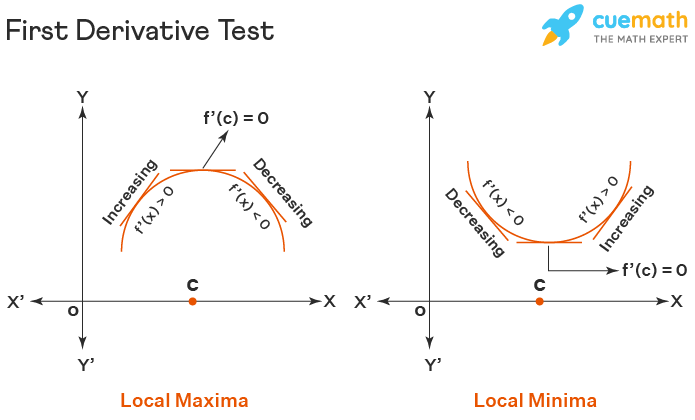
Let's formalize this.
Calculus I - The Shape of a Graph, Part I
Pauls Online Math Notes provides a clear, formal definition of the First Derivative Test.
Read the section titled First Derivative Test. Pay close attention to the three cases described. It's also important to note the distinction made between relative (or local) extrema and absolute extrema.
The process for finding and classifying local extrema is an extension of our previous one:
- Find the derivative .
- Find the critical points.
- Create a sign chart (number line) for .
- Determine intervals of increase and decrease.
- Apply the First Derivative Test at each critical point to classify it as a local maximum, local minimum, or neither.
A Comprehensive Example
Let's work through a more involved example that showcases the power and nuances of this test, especially when dealing with critical points where the derivative is undefined.
Consider the function . We want to find its intervals of increase and decrease and classify all local extrema.
Step 1: Find the derivative.
Using the power rule:
Step 2: Find the critical points.
To make this easier, let's factor the derivative. The common factor is .
Critical points occur where or is undefined.
- when the numerator is zero: .
- is undefined when the denominator is zero: .
So, our critical points are and .
Step 3 & 4: Create a sign chart and test intervals.
We divide the number line into three intervals: , , and .
| Interval | Test Value | Sign of | Behavior of |
|---|---|---|---|
| Increasing | |||
| Decreasing | |||
| Increasing |
Step 5: Apply the First Derivative Test.
- At , the derivative changes from positive to negative. Therefore, has a local maximum at . The value is .
- At , the derivative changes from negative to positive. Therefore, has a local minimum at . The value is .
This example is important because it shows that you must consider points where the derivative is undefined. The function has a sharp corner, or "cusp," at , but this point is still a local maximum.
Professor Leonard provides an excellent walkthrough of a very similar problem. Watching him solve it will help solidify this process.
Calculus 1 Lecture 3.3: The First Derivative Test for Increasing and Decreasing
Professor Leonard works through an example with fractional exponents, emphasizing the need to check for critical numbers from both the numerator and the denominator of the derivative.
Watch the segment from this example. Pay close attention to how he rewrites the derivative to clearly identify where it is zero and where it is undefined, and how both types of critical numbers are essential for the analysis.
Conclusion
In this lesson, we have developed one of the most practical tools in differential calculus. By analyzing the sign of the first derivative, we can now confidently map out the behavior of a function.
Key Takeaways:
- The sign of the first derivative tells you about the direction of the function: means is increasing, and means is decreasing.
- Critical points (where or is undefined) are the only places where a function can change from increasing to decreasing or vice versa.
- The First Derivative Test formalizes this analysis:
- A sign change from
+to-in indicates a local maximum. - A sign change from
-to+in indicates a local minimum. - No sign change means the critical point is not a local extremum.
- A sign change from
This skill is the first major step toward being able to sketch a detailed graph of a function without relying on a calculator. However, our sketches are still missing a key piece of information: the curvature or concavity of the graph. In our next lesson, we will introduce the second derivative and the Second Derivative Test, which will allow us to determine concavity and provide an alternative method for classifying extrema.