Rolle's and Mean Value Theorems

Rolle's Theorem: The Horizontal Case

As you saw in the video, Rolle's Theorem is a special case that is easy to understand intuitively. It deals with a "smooth" (differentiable) function that starts and ends at the same height over an interval. If you drive up a mountain and then back down to the same starting altitude, at some point, you must have been at a peak where the road was momentarily flat. That's the essence of Rolle's Theorem.

Formally, Rolle's Theorem has three conditions:

1. The function $f$ must be continuous on the closed interval $[a,b]$.
2. The function $f$ must be differentiable on the open interval $(a,b)$.
3. The function values at the endpoints must be equal, i.e., $f(a)=f(b)$.

If these conditions are met, the theorem guarantees that there is at least one number $c$ in the open interval $(a,b)$ such that $f^{\prime }(c)=0$.

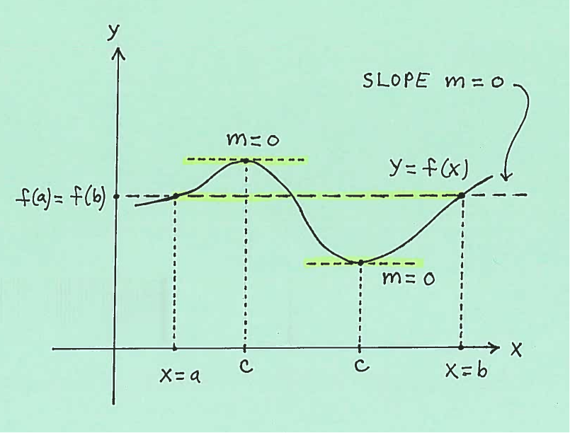
The conditions of continuity and differentiability are essential. If a function has a sharp corner (is not differentiable) or a break (is not continuous), we can't guarantee a point with a zero slope, even if the endpoints have the same value.

The following resource provides a formal statement of the theorem, a proof, and examples.

The Mean Value Theorem: The "Slanted" Case

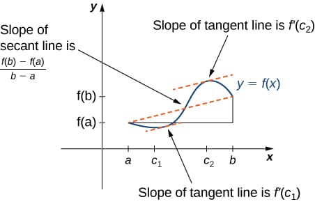
The Mean Value Theorem (MVT) is a powerful generalization of Rolle's Theorem. It drops the restrictive condition that $f(a)$ must equal $f(b)$. Instead of guaranteeing a horizontal tangent, it guarantees a tangent line that is parallel to the secant line connecting the endpoints.

In physical terms, if you travel 120 km in 2 hours, your average velocity is 60 km/h. The MVT guarantees that at some instant during your trip, your speedometer must have read exactly 60 km/h.

The MVT has two conditions:

1. The function $f$ must be continuous on the closed interval $[a,b]$.
2. The function $f$ must be differentiable on the open interval $(a,b)$.

If these conditions hold, then there exists at least one number $c$ in $(a,b)$ such that:

The left side of this equation is the instantaneous rate of change at point $c$. The right side is the average rate of change over the entire interval $[a,b]$. The MVT provides the crucial link between these two concepts.

Let's dive into the formal details and an application.

To see the complete process of verifying the hypotheses and finding the value of $c$, let's watch a worked example.

An Application: Proving the Number of Roots

Rolle's theorem is a surprisingly effective tool in proofs, particularly for showing that an equation has exactly one root in a given interval. The strategy combines the Intermediate Value Theorem (which we saw earlier) and Rolle's Theorem.

Let's see how to prove that the equation $f(x)=x^3+x-1$ has exactly one real root.

1. Existence of a root (IVT): First, we show there is at least one root. Notice that $f(0)=-1$ (negative) and $f(1)=1$ (positive). Since $f(x)$ is a polynomial, it's continuous everywhere. By the Intermediate Value Theorem, $f(x)$ must take on every value between -1 and 1, which includes 0. Therefore, there must be at least one root $d$ in the interval $(0,1)$.

2. Uniqueness of the root (Rolle's Theorem): Now, we show there cannot be more than one root. We do this by contradiction. Suppose there were two roots, $a$ and $b$. This would mean $f(a)=0$ and $f(b)=0$, so $f(a)=f(b)$. The function is a polynomial, so it's continuous and differentiable everywhere. Thus, it satisfies all three conditions for Rolle's Theorem on the interval $[a,b]$.

   Rolle's Theorem would then imply that there must be some number $c$ between $a$ and $b$ where $f^{\prime }(c)=0$. Let's check the derivative: $f^{\prime }(x)=3x^2+1$. Is it ever zero?

   $$3x^2+1=0⟹3x^2=-1⟹x^2=-1/3$$

   This equation has no real solutions, since the square of a real number cannot be negative. So, $f^{\prime }(x)$ is never zero. This contradicts the conclusion of Rolle's Theorem.

   Since our assumption (that there are two roots) led to a contradiction, the assumption must be false. Therefore, there cannot be more than one root.

Since there is at least one root and no more than one root, we can conclude there is exactly one root.

Conclusion

In this lesson, we explored two foundational theorems of calculus that connect the average and instantaneous rates of change. These theorems are not just theoretical curiosities; they are the bedrock upon which our methods for analyzing functions are built.

Key Takeaways:

• Rolle's Theorem is a special case for a differentiable function where $f(a)=f(b)$. It guarantees a point $c$ in $(a,b)$ where the tangent is horizontal ($f^{\prime }(c)=0$).
• The Mean Value Theorem (MVT) generalizes this. For any differentiable function, it guarantees a point $c$ where the instantaneous rate of change equals the average rate of change over the interval: $f^{\prime }(c)=\frac{f(b)-f(a)}{b-a}$.
• The key to applying these theorems is to first verify the hypotheses: the function must be continuous on the closed interval $[a,b]$ and differentiable on the open interval $(a,b)$.
• These theorems have important consequences. For instance, they allow us to prove properties about functions, such as the number of roots an equation has.

In our next lesson, we will look at the direct consequences of the MVT, which allow us to use the sign of the first derivative ($f^{\prime }$) to determine where a function is increasing or decreasing. This will give us our first powerful tool for sketching the graph of a function: the First Derivative Test.