Classifying Extrema with the Second Derivative Test

Introduction

In our previous lessons, we've developed a powerful toolkit for analyzing functions. We used the First Derivative Test to find where a function is increasing or decreasing and to locate its local extrema. Then, we used the Concavity Test to determine a function's curvature and find its inflection points by examining the second derivative.

Today, we'll connect these ideas. You've seen that a local maximum often occurs at the top of a "hill" (a region of downward concavity) and a local minimum at the bottom of a "valley" (a region of upward concavity). This lesson formalizes that intuition. We will introduce the Second Derivative Test, a convenient alternative to the First Derivative Test for classifying local extrema. This test uses the sign of the second derivative at a critical point, rather than the signs of the first derivative around it. This corresponds to the latter part of Section 4.3 in your Stewart textbook.

The Intuition Behind the Test

Let's begin by visualizing the connection. Suppose we have a critical point $c$ , where the tangent line is horizontal, meaning $f^{'} (c) = 0$ .

If the graph is concave upward at $c$ , it looks like the bottom of a valley. A horizontal tangent at the bottom of a valley corresponds to a local minimum.
If the graph is concave downward at $c$ , it looks like the top of a hill. A horizontal tangent at the top of a hill corresponds to a local maximum.

The following images illustrate this simple but powerful idea.

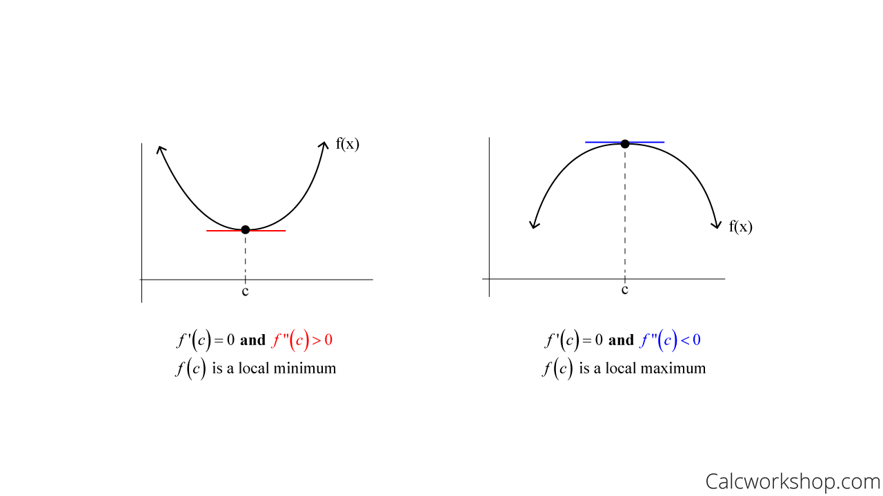
A visual summary of the Second Derivative Test. On the left, a horizontal tangent ($f'(c)=0$) on a concave up curve ($f''(c)>0$) indicates a local minimum. On the right, a horizontal tangent on a concave down curve ($f''(c)<0$) indicates a local maximum.

This relationship between the first derivative being zero and the sign of the second derivative is the heart of the test.

Formalizing the Second Derivative Test

Now, let's translate this visual intuition into a formal mathematical test. The resource below from the University of Texas provides a concise statement of the test and the logic behind it.

The Second Derivative Test

This document lays out the formal conditions of the test and provides two clear explanations for why it works.

Focus on the section titled "Second Derivative Test". Read the three bullet points that define the test for a local minimum/maximum and the inconclusive case. Then, read the two paragraphs immediately following, which explain the reasoning from both a concavity perspective and a rate-of-change perspective.

As you've just read, the Second Derivative Test is stated as follows:

Suppose $f^{''}$ is continuous near a point $c$ .

If $f^{'} (c) = 0$ and $f^{''} (c) > 0$ , then $f$ has a local minimum at $c$ .
If $f^{'} (c) = 0$ and $f^{''} (c) < 0$ , then $f$ has a local maximum at $c$ .
If $f^{'} (c) = 0$ and $f^{''} (c) = 0$ , the test is inconclusive.

This "inconclusive" case is extremely important. It does not mean there is no maximum or minimum; it simply means the Second Derivative Test fails to give an answer, and you must use a different method—namely, the First Derivative Test.

The Inconclusive Case: When the Test Fails

Why is the test inconclusive when $f^{''} (c) = 0$ ? Consider these three simple functions at $x = 0$ :

$f (x) = x^{4}$ : Here, $f^{'} (x) = 4 x^{3}$ and $f^{''} (x) = 12 x^{2}$ . At $x = 0$ , we have $f^{'} (0) = 0$ and $f^{''} (0) = 0$ . By observing the graph (a flattened parabola), we know there is a local minimum at $x = 0$ .
$f (x) = - x^{4}$ : Here, $f^{'} (x) = - 4 x^{3}$ and $f^{''} (x) = - 12 x^{2}$ . At $x = 0$ , we again have $f^{'} (0) = 0$ and $f^{''} (0) = 0$ . In this case, there is a local maximum at $x = 0$ .
$f (x) = x^{3}$ : Here, $f^{'} (x) = 3 x^{2}$ and $f^{''} (x) = 6 x$ . At $x = 0$ , we have $f^{'} (0) = 0$ and $f^{''} (0) = 0$ . This function has neither a maximum nor a minimum at $x = 0$ ; it has an inflection point.

Since all three outcomes (local min, local max, or neither) are possible when $f^{''} (c) = 0$ , the test provides no conclusion. In such cases, you must revert to the First Derivative Test by checking the sign of $f^{'} (x)$ on either side of the critical point $c$ .

Applying the Test: A Step-by-Step Procedure

Let's put this all together into a practical workflow.

Procedure for the Second Derivative Test:

Find the first derivative, $f^{'} (x)$ .
Find the critical numbers by setting $f^{'} (x) = 0$ and solving for $x$ . (This test only works for critical numbers where the tangent is horizontal, not where the derivative is undefined).
Find the second derivative, $f^{''} (x)$ .
For each critical number $c$ found in step 2, evaluate $f^{''} (c)$ .
- If $f^{''} (c) > 0$ , you have a local minimum at $c$ .
- If $f^{''} (c) < 0$ , you have a local maximum at $c$ .
- If $f^{''} (c) = 0$ , the test is inconclusive. Use the First Derivative Test.

The following video provides an excellent walkthrough of this process.

Second Derivative Test

The Organic Chemistry Tutor demonstrates how to apply the test to a polynomial function and confirms the result using the First Derivative Test.

Watch the first main example from this segment. Pay close attention to how the critical numbers are found first, and then the second derivative is used to classify them. Notice how he uses the concavity shapes (cup up/down) to remember which sign corresponds to a max or min.

First Derivative Test vs. Second Derivative Test

We now have two different tests for classifying local extrema. When should you use each one?

The First Derivative Test is more general. It works for any critical point (where $f^{'} (c) = 0$ or $f^{'} (c)$ is undefined) and is your required fallback when the Second Derivative Test is inconclusive. Its disadvantage is that it requires testing intervals on either side of the critical point.
The Second Derivative Test is often faster, especially if the second derivative is easy to compute. You only need to evaluate the sign of $f^{''} (x)$ at the critical point itself, not in the surrounding intervals. Its disadvantage is that it can be inconclusive and doesn't apply to critical points where the derivative is undefined.

The GeeksforGeeks article below provides a helpful summary of these differences and the limitations of the Second Derivative Test.

Second Derivative Test

This article includes a useful comparison table and a list of limitations.

First, review the comparison table to see a side-by-side summary of the two tests. Then, read the section on the Limitations, which reinforces the points about the inconclusive case and when the test cannot be applied.

Your choice of which test to use will often depend on the function. If finding $f^{''} (x)$ looks like it will be very complicated (e.g., it requires multiple applications of the quotient or product rule), it might be more efficient to just use the First Derivative Test from the start.

Conclusion

In this lesson, we've added the Second Derivative Test to our arsenal. It provides an efficient method for classifying local maxima and minima by linking them to the function's concavity at critical points.

Key Takeaways:

The Second Derivative Test is used to classify critical points where $f^{'} (c) = 0$ .
If $f^{''} (c) > 0$ (concave up), then $f (c)$ is a local minimum.
If $f^{''} (c) < 0$ (concave down), then $f (c)$ is a local maximum.
If $f^{''} (c) = 0$ , the test is inconclusive, and you must use the First Derivative Test to classify the critical point.
The Second Derivative Test is often quicker than the First Derivative Test, but it is less general and can fail.

You are now equipped with a complete set of tools for analyzing the local behavior of a function. In our next lesson, we will synthesize everything we've learned—increasing/decreasing intervals, concavity, inflection points, and local extrema—to achieve a major goal of differential calculus: sketching a detailed and accurate graph of a function from its equation alone.

Recommended resources