Hello! In our last lesson, we focused on simplifying complex rational expressions by finding the Least Common Denominator (LCD). This gave you a powerful tool for tidying up complicated fractions. Today, we'll take that skill a step further. Instead of just simplifying expressions, we will use the LCD to solve equations that contain algebraic fractions.
This is a crucial step in your algebraic toolkit. Many problems in calculus and machine learning, particularly in optimization, require you to set a rational expression equal to zero and solve for a variable. The method we'll cover today is the standard and most reliable way to do just that.
From Simplifying to Solving
In the previous lesson, to simplify an expression like , you learned to multiply the second term by to get a common denominator, resulting in . You couldn't simply multiply the whole expression by , as that would change its value.
The game changes with an equation, such as . Because of the equals sign, we can perform the same operation on both sides without changing the solution. This allows us to multiply both sides by the LCD to eliminate the denominators entirely, transforming a rational equation into a much simpler linear or quadratic equation.
The General Strategy for Solving Rational Equations
The overall process is systematic and builds directly on what you already know. The image below provides a great five-step summary of the method.
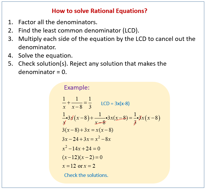
The most important and easily forgotten part of this process is the final step: checking your solutions. We'll soon see why this is absolutely critical.
For a gentle start, let's watch a short video that applies this logic to equations with numerical fractions. This will bridge the gap between familiar arithmetic and the algebraic problems we're about to tackle.
Solving Linear Equations with Fractions in Just Two Steps│Algebra
This video from GoTutor Math introduces a clear, two-step method for solving linear equations with fractions. It's a great warm-up for the algebraic versions we'll be handling.
Watch the introduction from the beginning to understand the two main steps. Then, watch the first example from the first example to see how multiplying by the LCM (our LCD) clears the fractions and leads to a simple linear equation.
Applying the Method to Rational Equations
Now, let's apply this same process to an equation with variables in the denominators. The core idea remains identical: find the LCD and multiply every term by it.
This text from Mathematics LibreTexts will formally define a rational equation and walk through a complete example that results in a linear equation.
First, read the brief introductory paragraphs at the start. Then, carefully study Example \PageIndex{1}, from the problem statement \dfrac { 1 } { x } + \dfrac { 2 } { x ^ { 2 } } = \dfrac { x + 9 } { 2 x ^ { 2 } } down to the solution x=5. Notice how multiplying by the LCD, 2x^2, clears all the fractions.
Expression vs. Equation: A Critical Distinction
This is the perfect moment to pause and highlight a common pitfall. The technique of multiplying by the LCD to eliminate fractions only works for equations. Trying to do this when simplifying an expression will lead to an incorrect result. The following resource provides an excellent side-by-side comparison.
This section clearly contrasts the correct procedure for an expression versus an equation. Internalizing this difference is key to avoiding common mistakes.
Find the heading Rational Expressions and Rational Equations. Study the text and the table that compares the three columns: the incorrect way to handle an expression, the correct way for an expression (using what you learned last lesson), and the correct way for an equation (using today's method).
Extraneous Solutions
We now come to the most important part of the process: checking your answer. When we multiply both sides of an equation by an expression containing a variable (like ), we are assuming that expression is not zero. If our final solution makes that expression zero, it creates a division-by-zero error in the original equation. Such a "solution" is called an extraneous solution and must be rejected.
The best practice is to determine the "restricted values" at the very beginning—any values of that would make any denominator zero. Any potential solution that matches a restricted value is extraneous.
Let's see this in action.
This reading will show you how multiplying by the LCD can lead to a quadratic equation and, more importantly, how to identify and discard an extraneous solution.
Start by reading the text just before Example \PageIndex{3}, which introduces the concept of extraneous solutions. Then, work through Example \PageIndex{3} in detail, from Step 1 to Step 4. Pay close attention to why x=5 is rejected as a solution.
When the Result is a Quadratic Equation
Sometimes, after clearing the denominators, you won't get a simple linear equation. Instead, you might end up with a quadratic equation (). The procedure is the same; you just have an extra step of solving the quadratic, usually by factoring.
This next resource provides a well-structured example of this scenario.
Solving Rational Equations | ChiliMath
This example from ChiliMath walks through a problem where clearing the denominators results in a quadratic equation that must be solved.
Scroll down to Example 10. Read through the entire solution, starting from the LCD determination all the way to solving the final factored equation. Notice the "Critical Step" where all terms are moved to one side to set the quadratic equation to zero.
A Special Case: Proportions and Cross-Multiplication
If your equation consists of a single fraction equal to another single fraction, like , it's called a proportion. In this specific case, you can use a shortcut called cross-multiplication. This means setting the products of the diagonals equal: . This is mathematically equivalent to multiplying both sides by the LCD (), but it can be faster.
Solving Linear Equations with Fractions in Just Two Steps│Algebra
This short segment visually demonstrates the cross-multiplication shortcut for solving proportions.
Watch the section from this segment that explains and demonstrates how cross-multiplication works.
A word of caution: while fast, cross-multiplication isn't always the best approach. If the denominators have common factors, it's often simpler to find the true LCD first, as this can prevent you from creating an overly complicated polynomial to solve. The LCD method always works, whereas cross-multiplication is a special-case shortcut.
Conclusion
Today you've bridged the gap between simplifying expressions and solving equations. By leveraging the LCD, you can systematically transform complex rational equations into familiar linear or quadratic forms.
Here are the essential takeaways:
- The Goal: To solve a rational equation, multiply every term on both sides by the LCD to eliminate all denominators.
- The Process: First, factor all denominators to find the LCD. Then, multiply, solve the resulting simplified equation, and check your work.
- Restricted Values: Before you start, identify any values of the variable that would make a denominator in the original equation zero.
- Extraneous Solutions: Any potential solution that matches a restricted value is extraneous and must be discarded.
- Expression vs. Equation: Remember, you can only clear denominators by multiplying both sides in an equation. This does not work for simplifying expressions.
In our next lesson, we will shift our focus from solving for exact values to working with ranges of values as we learn to solve linear inequalities and represent their solutions graphically.