Kernel Memory Bandwidth and Throughput Calculation

From Theory to Practice: The Roofline Model and Arithmetic Intensity

Before we dive into the metrics, let's solidify our understanding of why we are calculating these specific values. The goal is to place our kernel's performance within the context of the hardware's capabilities. The Roofline model is the perfect visualization for this.

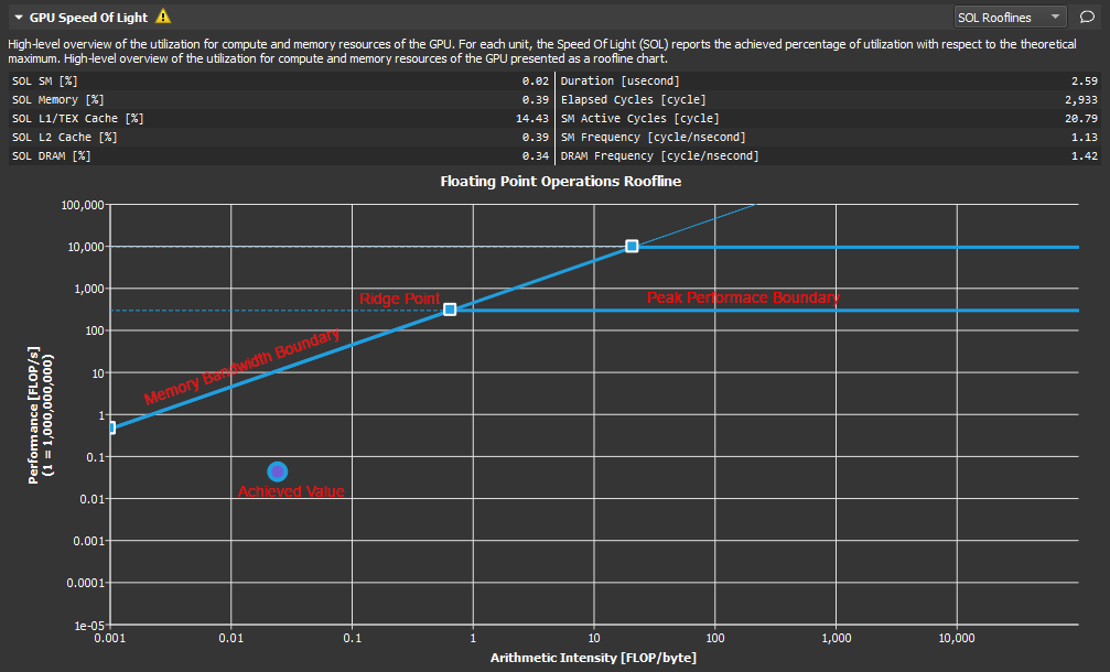
The x-axis, Arithmetic Intensity, is the ratio of work (floating-point operations) to data movement (bytes). The y-axis is the achieved performance, measured in Floating-Point Operations Per Second (FLOP/s). To calculate these two values, we need three key pieces of information about our kernel's execution:

1. Total FLOPs performed.
2. Total bytes transferred between the SMs and global memory (DRAM).
3. The total execution time (duration).

The following video provides an excellent conceptual breakdown of Arithmetic Intensity and how it's calculated for different types of algorithms. This will give you the intuition behind the formulas we'll use shortly.

Step 1: Collecting the Necessary Metrics with ncu

To get the raw data for our calculations, we must instruct Nsight Compute's command-line interface, ncu, to collect specific hardware performance counters. While the SOL view gives percentages, these low-level metrics provide the absolute counts we need.

The two main categories of metrics are for memory traffic and floating-point operations.

• Memory Traffic: We need to know how many bytes were read from and written to the GPU's main memory (DRAM). The metrics dram__sectors_read.sum and dram__sectors_write.sum count the number of 32-byte "sectors" transferred.
• Floating-Point Operations: We need to count the different types of floating-point instructions executed. Modern GPUs have specialized instructions, with the most common being FADD (addition), FMUL (multiplication), and the highly efficient FFMA (fused multiply-add).

The following article provides a clear, step-by-step guide on how to perform this data collection.

Step 2: Calculating Achieved Memory Bandwidth

Once you have run ncu with the correct metrics, you will have the raw data. Let's start by calculating the achieved memory bandwidth.

1. Calculate Total Bytes Transferred:
   The profiler gives us the number of DRAM sectors read and written. Since each sector on a modern NVIDIA GPU corresponds to a 32-byte transaction, the formula is:

   $$\text{Total Bytes}=(\text{dram\_\_sectors\_read.sum}+\text{dram\_\_sectors\_write.sum})\times 32$$

2. Find the Kernel Duration:
   The kernel's execution time, or duration, is reported directly by Nsight Compute in the SOL section. It's usually given in milliseconds (ms) or microseconds (µs). You'll need to convert this to seconds for our calculation. For example, 2.71 ms = 0.00271 s.

3. Calculate Bandwidth:
   Achieved memory bandwidth is the total bytes transferred divided by the time it took. To express this in the standard unit of gigabytes per second (GB/s), we use the following formula:

   $$\text{Achieved Bandwidth (GB/s)}=\frac{\text{Total Bytes}}{\text{Duration (s)}}\times 10^{-9}$$

Step 3: Calculating Achieved Compute Throughput

Next, let's calculate the rate at which our kernel performed floating-point operations, measured in GFLOPS/s (GigaFLOPs per second).

1. Calculate Total Floating-Point Operations (FLOPs):
   We sum the counts of the different operation types. Crucially, a single Fused Multiply-Add (FMA) operation (a * b + c) performs two floating-point operations (one multiplication, one addition), so we must count it twice.

   The formula for single-precision (FP32) FLOPs is:

   $$\text{Total FP32 FLOPs}=\text{fadd\_count}+\text{fmul\_count}+(2\times \text{ffma\_count})$$

   Where fadd_count is smsp__sass_thread_inst_executed_op_fadd_pred_on.sum, and so on for the other metrics you collected. If your kernel uses double-precision (FP64) or half-precision (FP16), you would use the corresponding metrics (e.g., dadd_count, dfma_count).

2. Calculate Throughput:
   Similar to bandwidth, the achieved compute throughput is the total FLOPs performed divided by the execution time. To get the result in GFLOPS/s:

   $$\text{Achieved Throughput (GFLOPS/s)}=\frac{\text{Total FLOPs}}{\text{Duration (s)}}\times 10^{-9}$$

A Practical Example: Quantifying an Optimization

Let's revisit the example from the SOL Analysis video, where a kernel was optimized by changing its data type from double (FP64) to float (FP32). In the last lesson, we saw this made the kernel faster. Now, let's quantify how and why.

Imagine we profile both versions and get the following (hypothetical but realistic) metrics:

Version 1: Double Precision (FP64)

• Duration: 2.71 ms (0.00271 s)
• dram__sectors_read.sum: 2,000,000
• dram__sectors_write.sum: 1,000,000
• smsp__sass_thread_inst_executed_op_dfma_pred_on.sum: 33,554,432 (This is the double-precision FMA counter)

Calculations for Version 1:

• Total Bytes = (2,000,000 + 1,000,000) * 32 = 96,000,000 bytes
• Achieved Bandwidth = (96,000,000 / 0.00271) / 1e9 ≈ 35.4 GB/s
• Total FP64 FLOPs = 2 * 33,554,432 = 67,108,864 FLOPs
• Achieved Throughput = (67,108,864 / 0.00271) / 1e9 ≈ 24.8 GFLOPS/s

Version 2: Float Precision (FP32)
After changing the code to use float, the data size is halved, and the GPU can use its much more numerous FP32 units.

• Duration: 63 µs (0.000063 s)
• dram__sectors_read.sum: 1,000,000
• dram__sectors_write.sum: 500,000
• smsp__sass_thread_inst_executed_op_ffma_pred_on.sum: 33,554,432 (This is the single-precision FMA counter)

Calculations for Version 2:

• Total Bytes = (1,000,000 + 500,000) * 32 = 48,000,000 bytes
• Achieved Bandwidth = (48,000,000 / 0.000063) / 1e9 ≈ 761.9 GB/s
• Total FP32 FLOPs = 2 * 33,554,432 = 67,108,864 FLOPs
• Achieved Throughput = (67,108,864 / 0.000063) / 1e9 ≈ 1065.2 GFLOPS/s

By performing these calculations, we've moved from "it's faster" to a precise, quantitative analysis: changing from double to float precision resulted in a ~43x speedup, increased memory bandwidth utilization by ~21x, and boosted compute throughput by ~43x. This demonstrates that the original kernel was severely limited by the GPU's scarce FP64 execution units, a bottleneck that the optimization completely removed, allowing the kernel to better utilize both the compute and memory subsystems.

Conclusion

In this lesson, you have learned to transform the raw hardware counter data from Nsight Compute into meaningful, quantitative performance metrics. This is a cornerstone skill for any performance engineer, allowing you to move beyond intuition and anchor your analysis in hard numbers.

Key Takeaways:

• To quantitatively analyze a kernel, you need its total FLOPs, total bytes transferred, and execution time.
• Nsight Compute (ncu) can collect the necessary low-level hardware counters for FLOPs (e.g., smsp__..._ffma_...) and memory traffic (e.g., dram__sectors_...).
• Achieved Memory Bandwidth (GB/s) is calculated by dividing total bytes transferred by the kernel duration.
• Achieved Compute Throughput (GFLOPS/s) is calculated by dividing total FLOPs by the kernel duration. Remember that FMA operations count as two FLOPs.
• These quantitative metrics allow for a precise comparison between different versions of a kernel, revealing the exact impact of an optimization.

You now possess the tools to calculate the coordinates of your kernel's performance. In our next lesson, we will complete the picture by learning how to construct a Roofline model for your GPU. We'll determine the "roofs"—the theoretical peak performance limits of your hardware—and plot your kernel's achieved performance against them. This will finally allow you to visualize exactly how much performance you are leaving on the table and guide your future optimization efforts.