Profiling Kernels with NVIDIA Nsight Compute

What is Nsight Compute?

Before diving in, it's important to understand what Nsight Compute is and where it fits in the ecosystem of performance tools. It is a kernel profiler. Its job is to give you an incredibly detailed view of what happens inside a single invocation of a single CUDA kernel. This is distinct from a system profiler (like Nsight Systems), which looks at the broader picture of how the CPU, GPU, and memory transfers interact over time.

For your goal of becoming a kernel engineer, Nsight Compute is the microscope you'll use to dissect and optimize the fine-grained behavior of your code. The following article provides an excellent overview of when and why you would reach for this tool.

As the article emphasizes, you use Nsight Compute when you want to know why a specific kernel is slow. It achieves this by collecting data from the GPU's hardware performance counters during the kernel's execution.

The Speed of Light (SOL) View: Your First Look

When you open an Nsight Compute report, the first and most important section you'll see is the GPU Speed of Light (SOL) summary. This section is designed to give you a high-level answer to the central question from our last lesson: is my kernel compute-bound or memory-bound?

It presents the utilization of the GPU's key resources as a percentage of their theoretical maximum performance. The two most prominent metrics are:

• SM Throughput (Compute Throughput): Indicates how busy the Streaming Multiprocessors' arithmetic units were. A high percentage suggests the kernel is performing a lot of computation.
• Memory Throughput: Indicates how much of the available DRAM bandwidth was used. A high percentage suggests the kernel is moving a lot of data to and from global memory.

The following video from NVIDIA provides an excellent walkthrough of this section. It explains what the SOL section is, what the key metrics mean, and how to interpret them to form an initial hypothesis about your kernel's performance.

By comparing the SM and Memory throughput percentages, you can make a quick, evidence-based assessment.

• High SM Throughput, Low Memory Throughput: The kernel is likely compute-bound. The arithmetic units are the bottleneck.
• Low SM Throughput, High Memory Throughput: The kernel is likely memory-bound. The memory system is the bottleneck.
• Low SM Throughput, Low Memory Throughput: This often indicates a latency-bound kernel. The GPU might be waiting for data from long-latency memory accesses, or there may not be enough parallel work to keep the hardware busy (low occupancy).
• High SM Throughput, High Memory Throughput: This is a "balanced" kernel, efficiently using both compute and memory resources. This is the ideal state, but it is rare.

Guided Analysis and Correlating to Source

Nsight Compute does more than just present data; it also provides Guided Analysis. This feature consists of a set of built-in "rules" that automatically analyze the collected metrics and provide plain-English explanations and suggestions. These rules are developed by NVIDIA's own performance engineers and effectively act as an expert system, pointing you toward potential problems.

A rule might trigger a warning like: "This kernel exhibits low compute throughput and memory bandwidth utilization..." and then suggest looking at other sections of the report for more details. This is an invaluable feature that helps you navigate the vast amount of data in a profile.

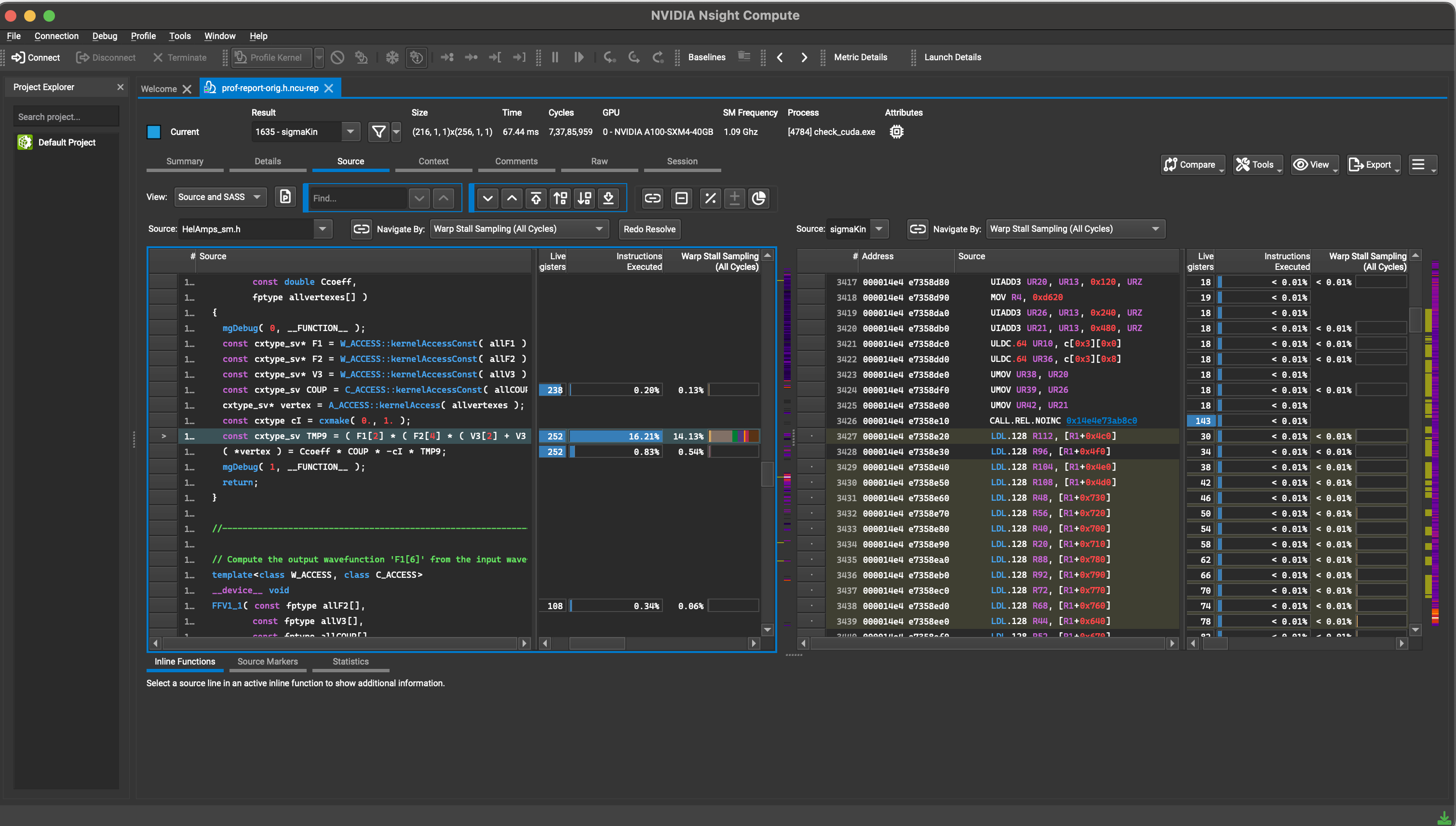
Perhaps the most powerful feature of Nsight Compute is its ability to correlate performance data directly back to your code. After identifying a high-level bottleneck (e.g., memory latency), you can switch to the Source page to see exactly which lines of your CUDA C++ code (and even the underlying assembly code) are responsible for the issue. This is where analysis becomes actionable.

The following video demonstrates these guided analysis and source correlation features.

A Practical Example: Fixing Uncoalesced Access

Let's walk through a concrete example. In Module 5, you learned about the importance of coalesced memory access. Let's see how Nsight Compute would diagnose a kernel with an uncoalesced access pattern.

Consider this kernel for 2D matrix addition, taken from the Profiling CUDA Kernels guide. It has a subtle but critical bug.

__global__ void matrix_add_2D_buggy(const arr_t* A, const arr_t* B, arr_t* C)
{
    // These indices are computed correctly for a 2D grid
    size_t idx = threadIdx.x + blockDim.x * (size_t)blockIdx.x;
    size_t idy = threadIdx.y + blockDim.y * (size_t)blockIdx.y;

    if ((idx < N) && (idy < N)) {
        // The BUG is here: the index related to threadIdx.x is used for the row, not the column.
        C[idx][idy] = A[idx][idy] + B[idx][idy];
    }
}

Threads in a warp have consecutive threadIdx.x values. For memory access to be coalesced, these threads should access consecutive memory locations. In C/C++, a 2D array C[row][col] is stored in row-major order. This means C[0][0], C[0][1], ..., C[0][N-1] are contiguous in memory.

In the code above, threads in a warp access C[idx][idy]. Since idx is derived from threadIdx.x, adjacent threads access C[0][idy], C[1][idy], C[2][idy], etc. These are elements in the same column, which are separated by an entire row's worth of bytes in memory. This is a classic uncoalesced access pattern.

How would Nsight Compute see this?

1. SOL View: You would likely see very high Memory Throughput. However, you'd also see warnings about memory efficiency. Nsight Compute would detect that the GPU is issuing many more memory transactions than necessary. Even though bandwidth is high, it's being used inefficiently. The SMs would likely be starved, leading to low SM Throughput. The primary bottleneck is memory latency and inefficiency.
2. Guided Analysis: A rule related to memory efficiency would fire. It would highlight a high ratio of memory transactions to memory requests, indicating that each request is being broken up into many small, inefficient transactions.
3. Source View: The profiler would highlight the line C[idx][idy] = A[idx][idy] + B[idx][idy]; as the source of high-latency global memory loads (ld.global). The stall metrics associated with this line would be very high, confirming it's where the kernel is spending most of its time waiting.

The fix, as you know from Module 5, is to swap the indices:

__global__ void matrix_add_2D_fixed(const arr_t* A, const arr_t* B, arr_t* C)
{
    size_t idx = threadIdx.x + blockDim.x * (size_t)blockIdx.x;
    size_t idy = threadIdx.y + blockDim.y * (size_t)blockIdx.y;

    if ((idx < N) && (idy < N)) {
        // FIXED: The index related to threadIdx.x is now the fastest-changing dimension.
        C[idy][idx] = A[idy][idx] + B[idy][idx];
    }
}

If you were to re-profile the fixed kernel, you would see a dramatic drop in kernel duration. The memory efficiency warnings would disappear, and you would see a much healthier balance between compute and memory throughput. The resource "Profiling CUDA Kernels with NVIDIA NSight Compute" walks through this exact scenario, showing how the number of memory sectors fetched per request drops from 32 down to 4 after the fix, confirming a massive improvement in efficiency.

Conclusion

You have now taken your first steps into the world of practical GPU performance analysis. While the Roofline Model gives you the theoretical lens, Nsight Compute provides the empirical data. You've learned how to approach a profiling report, starting from the high-level summary and drilling down to the specific lines of code that matter most.

Key Takeaways:

• Nsight Compute is the essential tool for diagnosing why a CUDA kernel is slow.
• The profiling workflow begins at the Speed of Light (SOL) section, which provides a high-level view of your kernel's relationship with the GPU's compute and memory subsystems.
• The comparison between SM Throughput and Memory Throughput gives you an immediate first guess at whether your kernel is compute-, memory-, or latency-bound.
• Guided Analysis Rules provide automated expertise, flagging common performance issues and directing your attention.
• The ultimate goal is to use the Source View to correlate performance bottlenecks directly to lines in your source code, making the problem actionable.

In our next lesson, we will bridge the gap between today's practical profiling and the previous lesson's theory. You will learn how to take the raw numbers from an Nsight Compute report and use them to calculate the achieved memory bandwidth and compute throughput of your kernel in concrete units (GB/s and GFLOPS/s), preparing you to plot your kernel on a Roofline chart.