Arithmetic Intensity and Kernel Classification

The Two Ceilings: Compute and Memory

Every program you run on a processor, whether a CPU or a GPU, is ultimately constrained by one of two physical limits: how fast it can perform calculations, or how fast it can feed the data required for those calculations. This is the central tension in high-performance computing.

The article "Mastering CUDA and High-Performance Computing, Part IV" eloquently describes this reality. I highly recommend reading the first two sections to set the stage. The author captures the essence of GPU performance engineering, which often has less to do with the arithmetic itself and more to do with the physics of moving data.

As the article highlights, there's a vast chasm between the processor's computational throughput (measured in FLOPS, or Floating-Point Operations Per Second) and its memory bandwidth (measured in Bytes per second). To understand which of these is limiting your kernel, we need a way to characterize the kernel's own demand for computation versus its demand for data.

Defining Arithmetic Intensity

We can formalize this relationship using a simple but powerful model. To start, let's watch a short video that introduces the core concepts from first principles.

As explained in the video, we can characterize any computational task by two numbers:

1. The total number of floating-point operations it performs (Work, or FLOPs).
2. The total volume of data it moves to and from main memory to perform those operations (Bytes).

From these, we define Arithmetic Intensity (AI), often denoted by $I$:

The unit of arithmetic intensity is FLOPs/Byte. It tells you, on average, how many calculations your algorithm performs for every single byte it fetches from or stores to global memory. A high AI means the algorithm does a lot of computation on its data, while a low AI means the algorithm is mostly just moving data around.

The Roofline Model: Visualizing Performance Limits

The arithmetic intensity of your kernel, combined with the hardware's peak performance and memory bandwidth, determines its theoretical maximum performance. This relationship is captured in the Roofline Model.

The model states that a kernel's attainable performance $P$ (in FLOPs/second) is limited by the minimum of two values: the machine's peak compute throughput and the performance achievable given the machine's memory bandwidth.

Where:

• $P_{\text{peak}}$ is the theoretical peak performance of the GPU (e.g., in TFLOPS/s). This is a fixed hardware characteristic.
• $I$ is the arithmetic intensity of your kernel (in FLOPs/Byte).
• $\beta$ (beta) is the peak memory bandwidth of the GPU (e.g., in GB/s or TB/s). This is also a fixed hardware characteristic.

This simple equation gives us a powerful classification tool. We can visualize it as a plot with Arithmetic Intensity on the x-axis and Performance (GFLOPS/s) on the y-axis.

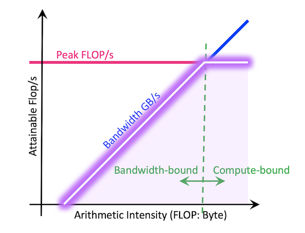
The plot shows two distinct regions:

• Memory-Bound Region (Slanted Line): When the arithmetic intensity $I$ is low, the performance is limited by $I\times \beta$. The kernel is "starved for data," and its speed is dictated by how fast the memory system can deliver bytes. We call such kernels memory-bound.
• Compute-Bound Region (Flat Line): When the arithmetic intensity $I$ is high, the performance hits a ceiling at $P_{\text{peak}}$. The memory system can supply data fast enough to keep the arithmetic units fully busy. We call such kernels compute-bound.

The "knee" of the roofline plot, where the two lines intersect, is known as the ridge point. This represents the minimum arithmetic intensity a kernel must have to be able to saturate the machine's compute units.

Calculating Arithmetic Intensity in Practice

Let's apply this by calculating the AI for two familiar operations: vector addition and matrix multiplication. The article from Vrushank Desai provides a very clear, step-by-step calculation.

Let's summarize the findings from the reading.

Example 1: Vector Addition (C = A + B)

This is the quintessential memory-bound operation. For each element of the output vector C, a kernel must:

1. Read one element from vector A.
2. Read one element from vector B.
3. Perform one addition operation.
4. Write one element to vector C.

Assuming 32-bit floats (4 bytes each):

• FLOPs per element: 1
• Bytes per element: 4 (read A) + 4 (read B) + 4 (write C) = 12 bytes
• Arithmetic Intensity (I): $\frac{1\text{ FLOP}}{12\text{ Bytes}}\approx 0.083$ FLOPs/Byte.

This is an extremely low AI. On virtually any modern GPU, this kernel will be heavily memory-bound. Optimizing the addition instruction itself is pointless; performance is entirely determined by memory bandwidth.

Example 2: Naive Matrix Multiplication (C = A * B)

Consider multiplying two $N\times N$ matrices.

1. Work (FLOPs): To compute each of the $N^2$ elements in the output matrix C, we perform a dot product of an N-element row and an N-element column. This requires $N$ multiplications and $N-1$ additions, for a total of $2N-1$ FLOPs. The total work is thus $N^2\times (2N-1)\approx 2N^3$ FLOPs.
2. Data (Bytes): In a naive implementation where we load all data from global memory, we must read matrix A ($N^2$ elements) and matrix B ($N^2$ elements), and write matrix C ($N^2$ elements). Total elements moved: $3N^2$. With 4-byte floats, this is $12N^2$ bytes.

The arithmetic intensity is:

This is a fascinating result. Unlike vector addition, the AI of matrix multiplication grows linearly with the problem size, N.

• For a small matrix (e.g., N=32), $I\approx 5.3$ FLOPs/Byte. This might still be memory-bound.
• For a large matrix (e.g., N=1024), $I\approx 170$ FLOPs/Byte. This is a very high AI and is almost certainly compute-bound.

This explains why optimizing GEMM (General Matrix Multiplication) is so important and effective in deep learning. Large matrix multiplies have enough arithmetic intensity to keep the GPU's powerful compute units fed, making them a prime target for compute-focused optimizations—a topic we will dedicate an entire future module to.

Conclusion

In this lesson, you have learned the fundamental concept of arithmetic intensity and its role in performance analysis. This framework allows you to move beyond guesswork and begin scientifically diagnosing why a kernel performs the way it does.

Key Takeaways:

• A kernel's performance is limited by either its computational requirements or its memory access requirements.
• Arithmetic Intensity (AI) is the ratio of FLOPs performed to bytes transferred from main memory ($I=\text{FLOPs}/\text{Bytes}$). It is the defining characteristic of an algorithm's performance profile.
• The Roofline Model provides a visual framework for understanding these limits, showing that attainable performance is the minimum of the hardware's peak compute rate and the bandwidth-limited rate ($\min (P_{\text{peak}},I\times \beta )$).
• Kernels with low AI (e.g., vector addition) are memory-bound. Their performance is dictated by memory bandwidth.
• Kernels with high AI (e.g., large matrix multiplication) are compute-bound. Their performance is dictated by the raw compute power of the processor.

Knowing whether your kernel is memory-bound or compute-bound is the first step in optimization. If you are memory-bound, you should focus on reducing memory traffic (e.g., through better data reuse with shared memory). If you are compute-bound, you focus on increasing instruction throughput.

In our next lesson, we will make this theory practical. You will learn how to use NVIDIA Nsight Compute, a professional profiling tool, to measure the actual performance and memory traffic of a kernel, calculate its achieved arithmetic intensity, and begin constructing your first roofline plot to visualize its bottlenecks.