Roofline Modeling for GPU Performance Analysis

Introduction

In our last lesson, you learned the crucial skill of calculating a kernel's achieved performance, turning raw profiler counters into concrete metrics like GFLOPS/s and GB/s. These values represent your kernel's actual performance—the "y-coordinate" on a performance graph. Now, it's time to build the rest of that graph.

This lesson focuses on constructing a Roofline model, a powerful tool for visualizing performance. You will learn how to determine the theoretical hardware limits of a GPU—its peak compute throughput and memory bandwidth—and plot them as "roofs" that bound all possible performance. By placing your kernel's previously calculated performance point on this chart, you will be able to instantly diagnose whether it is limited by computation or memory access, and, just as importantly, see exactly how much performance you are leaving on the table. This model transforms performance analysis from a guessing game into a systematic engineering discipline.

The Anatomy of the Roofline Model

At its core, the Roofline model simplifies a complex processor into two key numbers: its peak computational rate and its peak memory bandwidth. It then plots performance against arithmetic intensity, the ratio of work to data movement you're already familiar with.

To build our understanding from first principles, let's watch a short video that introduces the fundamental concepts of the Roofline model.

A very short intro to the Roofline model

This video, "A very short intro to the Roofline model" from NHR@FAU, provides a clear, step-by-step derivation of the model.

Please watch the following sections: The simple hardware and software view: This explains how the model abstracts the hardware into peak performance (P_{peak}) and bandwidth (B_s), and the software into a single number: computational intensity (I). The two bottlenecks: This section derives the core Roofline equation: P = \min(P_{peak}, I \cdot B_s). This is the mathematical foundation of the entire model. Plotting the model: Here, you'll see how the equation is visualized as two lines on a log-log plot, creating the characteristic "roof" shape and the all-important "knee" or ridge point.

As the video explains, the model presents an upper bound on performance. Your kernel is either limited by how fast it can compute or by how fast it can be fed data. The lower of these two limits is the one that applies.

Step 1: Characterizing the Hardware (Constructing the Roofs)

To build a Roofline chart, we first need to define the hardware's capabilities. This involves finding the two peak values for our target GPU.

The Compute Roof ( $P_{p e ak}$ )

This is a horizontal line on the chart representing the theoretical maximum number of floating-point operations per second the GPU can execute. This value depends heavily on the data type (e.g., FP32, FP64, FP16/BF16) and whether specialized units like Tensor Cores are used.

The Memory Roof ( $B_{p e ak}$ )

This is a sloped line on the chart. Its slope is equal to the peak memory bandwidth of the GPU's High Bandwidth Memory (HBM). It represents the performance limit for a kernel that has to move a certain amount of data for its computations. The performance is given by $P = B_{p e ak} \cdot I$ .

The following resource provides a concise guide to these concepts and grounds them with specifications from a real-world GPU, the NVIDIA A100.

Learn about Roofline Model - Mojo GPU Puzzles

This article offers a practical and clear explanation of the Roofline model's components.

Please read the first three sections of the article: Introduction: This sets the stage, framing the Roofline model as a "compass for GPU optimization." The two ceilings: Pay close attention to the definitions of the memory and compute roofs and the formula for critical intensity, which we'll discuss next. Hardware example: This section provides concrete numbers for an A100 GPU, showing you exactly where the P_{peak} and B_{peak} values come from.

The Ridge Point: Machine Balance

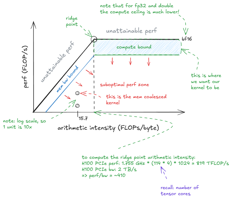
The intersection of the compute roof and the memory roof is called the ridge point or knee. The arithmetic intensity at this point is the critical intensity, $I^{*}$ .

I^{*} = \frac{P _{p e ak}}{B _{p e ak}}

This value represents the "balance" of the machine.

If your kernel's arithmetic intensity $I$ is less than $I^{*}$ , it lies to the left of the ridge point. The performance ceiling above it is the memory roof. The kernel is memory-bound.
If your kernel's arithmetic intensity $I$ is greater than $I^{*}$ , it lies to the right of the ridge point. The performance ceiling is the compute roof. The kernel is compute-bound.

This distinction is the primary diagnostic output of the Roofline model. It tells you exactly what class of optimizations to pursue.

A conceptual diagram of the Roofline model. Kernels with low arithmetic intensity fall in the 'mem bw bound' region, while those with high intensity fall in the 'compute bound' region. The goal of many optimizations is to increase arithmetic intensity (move right) and/or improve hardware utilization (move up) to get closer to the performance ceiling.

Step 2: Plotting Your Kernel's Performance

Now that we have the "roof," we can plot our kernel's achieved performance on the chart. As you learned in the previous lesson, you already know how to calculate the two coordinates for this point:

X-coordinate (Arithmetic Intensity): $I = \frac{Total FLOPs}{Total Bytes Transferred}$
Y-coordinate (Achieved Performance): $P_{a c hi e v e d} = \frac{Total FLOPs}{Execution Time}$

Let's put this all together with a practical example.

Scenario:

Hardware: A simplified GPU with $P_{p e ak}$ = 20 TFLOP/s (FP32) and $B_{p e ak}$ = 1,000 GB/s.
Kernel: A simple vector addition kernel, vec_add(float* a, float* b, float* c, int n).

Analysis:

Construct the Roofline:
- Compute Roof: A horizontal line at $P = 20, 000$ GFLOP/s.
- Memory Roof: A line with slope 1,000 GB/s.
- Critical Intensity ( $I^{*}$ ): $I^{*} = \frac{20 \times 1 0 ^{12} FLOP/s}{1000 \times 1 0 ^{9} B/s} = 20 FLOP/Byte$
Analyze the Kernel:
- For each element, we perform 1 add operation (1 FLOP).
- We read two floats (8 bytes) and write one float (4 bytes), for a total of 12 bytes of memory traffic per element.
- Kernel's Arithmetic Intensity ( $I$ ): $I = \frac{1 FLOP}{12 Bytes} \approx 0.083 FLOP/Byte$
Plot and Diagnose:
- Our kernel's intensity $I \approx 0.083$ is far less than the critical intensity $I^{*} = 20$ . The kernel is deep in the memory-bound region.
- The theoretical maximum performance for this kernel is determined by the memory roof: $P_{ma x} = I \cdot B_{p e ak} = 0.083 FLOP/B \times 1000 GB/s \approx 83 GFLOP/s$
- This is the point on the roof directly above our kernel's x-coordinate. It represents only $83/20, 000 \approx 0.4%$ of the GPU's peak compute performance!
- If you then profiled the kernel and found its achieved performance was, say, 70 GFLOP/s, you could plot the point $(0.083, 70)$ . The small vertical gap between your point and the memory roof (at 83 GFLOP/s) indicates you are getting good memory bandwidth utilization, but the huge horizontal gap to the ridge point shows that the kernel's nature is the primary performance limiter.

From Manual Calculation to Automated Tools

Manually calculating FLOPs and bytes is essential for understanding the principles, but for complex applications, profilers can automate this process. NVIDIA's Nsight Compute has a built-in Roofline analysis feature that does exactly this.

The following resource explains how to use such tools and introduces the concept of a hierarchical Roofline model, which includes ceilings for different cache levels (L1, L2), providing even deeper insight.

Roofline Performance Model - NERSC Documentation

This document from the NERSC documentation provides a comprehensive overview of the Roofline model and its practical application.

Please read the following sections: Roofline Performance Model: This provides a formal definition and reinforces the interpretation of memory-bound vs. compute-bound regions. Hierarchical Roofline: Briefly read this part to understand that we can create separate roofs for L1 and L2 cache, which is crucial for analyzing optimizations like shared memory tiling. Application Characterization: This section explicitly lists the three pieces of data needed, reinforcing what you learned in the last lesson. Note the mention of Nsight Compute as an automated tool. Arithmetic Intensity: This part connects directly to our last lesson, showing how profiler metrics like dram_read_transactions are used to calculate total bytes, just as you learned.

The output of a tool like Nsight Compute generates a chart very similar to our theoretical one, but with measured, attainable hardware peaks and your kernel's achieved performance plotted automatically.

An actual Roofline analysis graph from NVIDIA Nsight Compute. The tool calculates the kernel's Arithmetic Intensity and Performance (the blue dot) and plots it against the device's compute (horizontal lines) and memory (diagonal line) ceilings.

Conclusion

You have now completed the conceptual loop of performance analysis. You started by getting a qualitative feel with SOL, then learned to calculate quantitative performance metrics, and now you can place those metrics in the context of the hardware's theoretical limits using the Roofline model.

Key Takeaways:

The Roofline model visualizes performance limits set by a GPU's peak compute throughput ( $P_{p e ak}$ ) and peak memory bandwidth ( $B_{p e ak}$ ).
The performance of any kernel is bounded by $P_{a c hi e v ab l e} = min (P_{p e ak}, I \cdot B_{p e ak})$ .
The critical intensity ( $I^{*} = P_{p e ak} / B_{p e ak}$ ) is the "machine balance" point that separates memory-bound kernels ( $I < I^{*}$ ) from compute-bound kernels ( $I > I^{*}$ ).
Plotting a kernel's (Arithmetic Intensity, Achieved Performance) point on the model immediately diagnoses its primary bottleneck and shows the headroom for optimization.
To improve a memory-bound kernel's performance, you must either increase its arithmetic intensity (e.g., by improving data reuse) or improve its memory bandwidth utilization.

In our next lesson, we will put this powerful diagnostic tool to work. We will begin the iterative optimization cycle: profile a kernel, use the Roofline model to identify its bottleneck, formulate a hypothesis for an optimization, implement it, and then re-profile to measure the impact. The Roofline chart will be our guide, showing us how our changes move the kernel's performance point up and to the right.

Recommended resources