Introduction
In our previous lesson, we established the Roofline model as a powerful diagnostic tool. By plotting a kernel's performance against the hardware's theoretical limits, we can instantly determine if it is memory-bound or compute-bound. This diagnosis is the critical first step, but it's only half the story. The true work of a kernel engineer lies in the systematic process of turning that diagnosis into measurable performance gains.
This lesson introduces the formal methodology for that process: iterative, analysis-driven optimization. You will learn to apply a structured cycle of profiling a kernel, identifying its primary bottleneck, forming a hypothesis for an optimization, implementing that change, and then re-profiling to measure the impact and uncover the next bottleneck. This loop is the fundamental workflow for high-performance computing. We will explore this concept, known in NVIDIA's terminology as the APOD (Assess, Parallelize, Optimize, Deploy) cycle, and see how it transforms performance tuning from an art into a repeatable science.
The Analysis-Driven Optimization Cycle
The core of modern performance engineering is a cyclical process. You don't simply "optimize" a kernel once. Instead, you chip away at successive performance limiters, with each fix revealing the next, smaller bottleneck. The CUDA Best Practices Guide formalizes this as the APOD cycle.
CUDA C++ Best Practices Guide 13.1 documentation
This guide introduces NVIDIA's official framework for GPU application development and optimization.
Please read the following sections to understand the high-level strategy: Assess, Parallelize, Optimize, Deploy: This introduces the full APOD cycle. Our focus in this lesson is on the "Optimize" phase, which is itself an iterative mini-cycle. The Optimization Process: This passage describes the core loop we will be studying: identify, apply, test, and repeat. Overall Performance Optimization Strategies: This provides a high-level summary of the types of optimizations we can apply within the cycle, which you've already encountered: maximizing parallelism, optimizing memory, and optimizing instructions.
The "Optimize" step described in the guide can be expanded into the clear, repeatable workflow that is the focus of this lesson:
- Assess (Profile): Run the application under a profiler like Nsight Compute to gather baseline performance data.
- Identify Bottleneck: Analyze the profiler data. Use the Roofline model, the Speed-of-Light (SOL) section, and warp state statistics to determine the primary factor limiting performance (e.g., memory bandwidth, compute latency, instruction fetch).
- Formulate Hypothesis: Based on the bottleneck, propose a specific, testable change. For example: "The kernel is memory-bound due to strided global memory access. Tiling the operation using shared memory will enable coalesced access and increase effective bandwidth."
- Implement Optimization: Modify the CUDA C++ code to implement the change.
- Re-Assess (Re-profile): Profile the modified code and compare the new performance against the baseline. Did performance improve as expected? What is the new bottleneck?
This loop continues until performance is "good enough" or is verifiably close to the hardware's theoretical maximum for that operation. The following flowchart illustrates how Nsight tools facilitate this process, with our focus being the iterative loop within Nsight Compute.
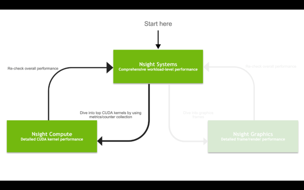
A typical optimization workflow starts with system-level analysis in Nsight Systems, then dives into detailed kernel analysis in Nsight Compute. The core optimization work involves iteratively profiling and modifying the kernel within Nsight Compute before re-checking overall performance.
A Practical Example: The Compute-Bound Kernel
Let's walk through a complete optimization cycle using a clear, practical example. The following video demonstrates how to use Nsight Compute to diagnose and fix a compute-bound kernel.
SOL Analysis with NVIDIA Nsight Compute | CUDA Developer Tools
This video from the NVIDIA Developer channel, "SOL Analysis with NVIDIA Nsight Compute," is a perfect demonstration of a single, complete optimization iteration.
As you watch, mentally map the presenter's actions to the five steps of our optimization cycle: Assess & Identify (Initial Analysis): The video begins by explaining the SOL section and then profiles a kernel that uses double precision floating-point numbers. Pay close attention to how the presenter interprets the SOL report. Note the high "Compute (SM) Throughput" and low "Memory Throughput." The "Compute Throughput Breakdown" further pinpoints the FP64 (64-bit floating point) pipe as the "long pole" or primary bottleneck. Formulate Hypothesis (The Hypothesis): The presenter correctly identifies that the specific GPU being used (a GeForce GTX 1660 Ti) has very limited FP64 performance compared to its FP32 performance. The hypothesis is simple: switching the computation from double to float should dramatically increase performance by moving the workload to the GPU's more powerful 32-bit floating-point units. Implement & Re-assess (Verification): The code is recompiled to use the float variant. The presenter then re-profiles and uses the "baselines" feature in Nsight Compute to directly compare the "before" and "after" results. Observe the massive (>97%) reduction in kernel duration and how the new kernel is now "balanced," with both compute and memory utilization being relatively high.
This example is a masterclass in the iterative methodology. The profiler didn't just say "the code is slow." It provided specific data pointing to the FP64 units as the bottleneck. This allowed for a precise, targeted optimization that yielded a dramatic speedup. The re-profiling step was essential to confirm the hypothesis and to see that the bottleneck had shifted.
Peeling the Performance Onion: A Multi-Step Journey
Rarely does a single optimization take a kernel from naive to perfect. More often, performance tuning is like peeling an onion: solving one bottleneck reveals the next, slightly smaller one.
Let's look at a more extended example using a matrix multiplication kernel, a problem central to AI and one you'll study in depth later. The following video demonstrates four successive optimization iterations.
CUDA Crash Course: GPU Performance Optimizations Part 1
This "CUDA Crash Course" video provides a fantastic demonstration of iterative optimization on a GEMM kernel.
Observe how each optimization addresses a different bottleneck revealed by the previous step: Iteration 1: Reducing Global Memory Writes (From 13s to 5s). The baseline writes intermediate results directly to slow global memory inside a loop. Hypothesis: Accumulating results in a fast register and writing to global memory only once will reduce memory traffic. The result is a massive speedup from 13s to 5s. Iteration 2: Coalescing Memory Accesses (From 5s to 4.25s). The new bottleneck is inefficient memory access. The thread block dimensions cause threads in a warp to access different rows of memory, leading to memory divergence. Hypothesis: Changing the block dimensions to align with the warp size (32) will result in coalesced memory accesses. This shaves off another second. Iteration 3: Vectorized Loads (From 4.25s to 3.5s). Now that accesses are coalesced, the bottleneck becomes underutilization of the memory bus width. Hypothesis: Using a vectorized data type like int4 will allow a single instruction to load four elements at once, increasing memory bandwidth utilization. This yields another significant gain. Iteration 4: Compiler-Assisted Unrolling (From 3.5s to 3.36s). The gains are getting smaller. The remaining bottleneck is minor loop overhead. Hypothesis: Instructing the compiler with #pragma unroll will eliminate loop control instructions. This provides a final, small improvement. The video even concludes by showing that this highly-optimized global memory version outperforms a naive shared memory implementation, driving home the point that applying optimization principles systematically is more important than blindly using "advanced" features. Knowing When to Stop This iterative process raises a crucial question for any engineer: How do you know when you're done? The answer lies in comparing your achieved performance to the theoretical limits we discussed in the Roofline lesson. You are "done" when one of two conditions is met: The performance is sufficient for the application's requirements. The achieved performance is very close to the theoretical Roofline for your kernel's arithmetic intensity, indicating there is little-to-no headroom left. Let's examine how a professional engineer makes this determination.
Knowing When to Stop
This iterative process raises a crucial question for any engineer: How do you know when you're done? The answer lies in comparing your achieved performance to the theoretical limits we discussed in the Roofline lesson.
You are "done" when one of two conditions is met:
- The performance is sufficient for the application's requirements.
- The achieved performance is very close to the theoretical Roofline for your kernel's arithmetic intensity, indicating there is little-to-no headroom left.
Let's examine how a professional engineer makes this determination.
Finishing the Analysis with NVIDIA Nsight Compute, Part 3
This NVIDIA developer blog post walks through the final, more advanced stages of an optimization process.
Please read these sections to understand how to determine when a kernel is "optimal enough": First Optimization: The author starts with a kernel limited by shared memory pressure and applies a warp-shuffle optimization, which relieves that pressure. The new bottleneck, identified by Stall Long Scoreboard, is global memory latency. Refactoring with cuBLAS: Facing a memory latency bottleneck, the author performs a major refactoring, splitting the kernel and using a highly optimized library (cuBLAS) for part of the work. This results in another large speedup. Is the global load optimal?: This is the key section. To determine if the remaining kernel is optimal, the author calculates its achieved bandwidth (823 GB/s). They then run the CUDA bandwidthTest sample to get a proxy for the GPU's maximum achievable bandwidth (740 GB/s). Since the achieved bandwidth is at or even slightly above this practical peak, they can confidently conclude the kernel's memory access is optimal and that further tuning is not worthwhile.
This final step closes the loop. You use the profiler to guide your changes, and you use theoretical and practical hardware limits to know when the optimization journey for a particular kernel has come to an end.
Conclusion
You have now learned the complete, end-to-end workflow for performance engineering. This iterative methodology is the engine of high-performance computing, providing a structured way to transform a slow, naive kernel into a highly tuned piece of code that pushes hardware to its limits.
Key Takeaways:
- GPU optimization is not a single action but an iterative cycle: Assess, Identify Bottleneck, Formulate Hypothesis, Implement, and Re-assess.
- This process is often called analysis-driven optimization because each step is guided by concrete data from profilers like Nsight Compute.
- Solving one bottleneck (e.g., compute limitation) will often reveal a new, more subtle one (e.g., memory access patterns), a process akin to "peeling an onion."
- The optimization process ends when performance is sufficient or when the kernel's achieved performance is demonstrably close to the theoretical hardware limits defined by the Roofline model.
In the next module, we will put this methodology into practice on a grand scale. You will embark on the classic journey of optimizing General Matrix Multiplication (GEMM), applying these iterative steps to build a high-performance kernel from the ground up, one optimization at a time.