Gradients for Layer Normalization

Introduction

In our previous lesson, we built a high-performance CUDA kernel for the Layer Normalization forward pass. We focused on fusing the mean and variance calculations with the normalization step, leveraging the numerically stable Welford's algorithm to do so in a single pass. This gave us a fast and accurate way to compute the layer's output.

Now, we must address the other half of the puzzle: the backward pass. To train a neural network, we need to propagate gradients back through the network to update the weights. This means that for our Layer Normalization layer, we need to calculate how a change in the loss function, represented by the incoming gradient $\frac{\partial l}{\partial y}$ , is attributable to the layer's inputs $x$ and its learnable parameters, $γ$ (scale) and $β$ (bias). This lesson is dedicated to deriving the mathematical formulas for these gradients. This theoretical groundwork is an essential prerequisite before we can implement the backward pass kernel in our next session.

The Layer Normalization Computation Graph

To derive the gradients, we'll use the chain rule from multivariable calculus. The most systematic way to do this is to first decompose the Layer Normalization operation into a sequence of simpler steps, forming a computation graph. This allows us to backpropagate the gradient one step at a time.

Recall the Layer Normalization formula for a single feature vector $x$ in a batch:

y_{i} = γ_{i} \frac{x _{i} - μ}{σ ^{2} + ϵ} + β_{i}

where $μ$ and $σ^{2}$ are the mean and variance calculated across all features for that specific input in the batch.

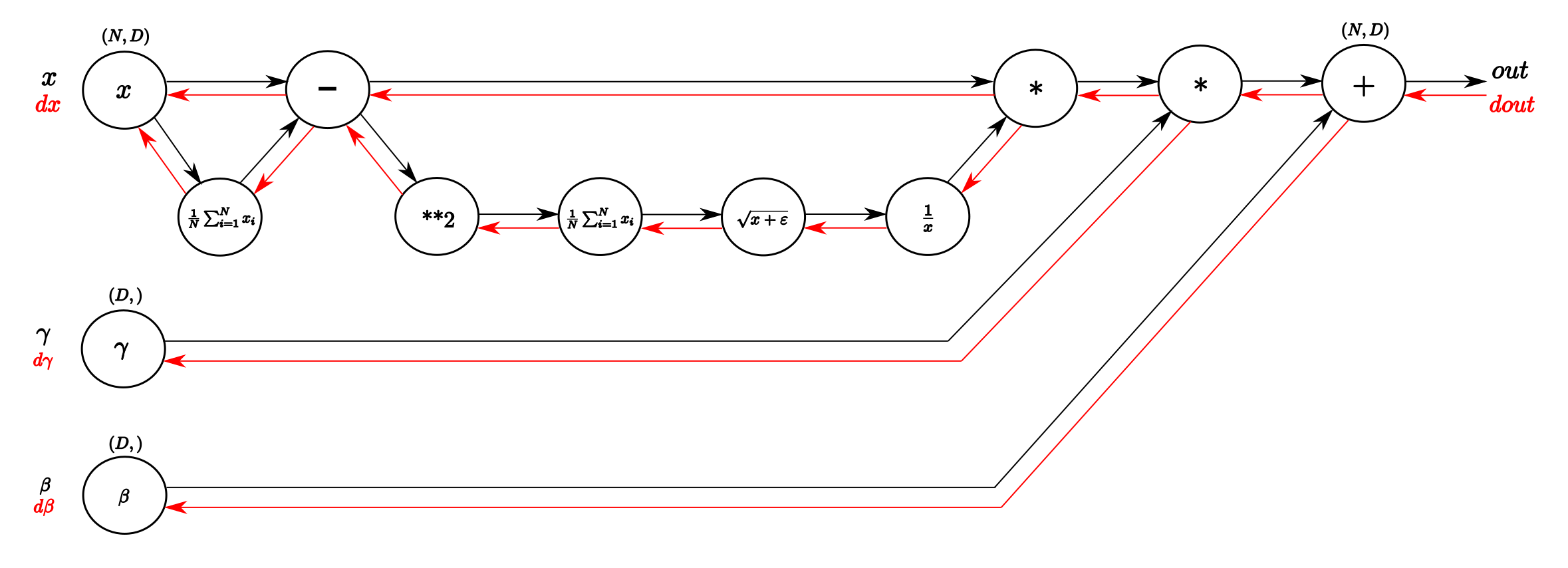
This diagram illustrates the forward and backward flow of information in a computation graph for Batch Normalization. The structure is analogous to Layer Normalization. The forward pass (black arrows) computes the output, while the backward pass (red arrows) propagates the gradients from the output back to the inputs.

To facilitate the derivation, let's break down the formula into intermediate variables, just as the robotchinwag.com article suggests. For a batch of inputs $X$ with shape ( $B$ , $H$ ), where $B$ is the batch size and $H$ is the number of features:

Mean: $m_{b} = \frac{1}{H} \sum_{h = 1}^{H} x_{bh}$
Centered Input: $μ_{bh} = x_{bh} - m_{b}$
Variance: $v_{b} = \frac{1}{H} \sum_{h = 1}^{H} (μ_{bh})^{2}$
Standard Deviation: $σ_{b} = v_{b} + ϵ$
Normalized Input: $x^_{bh} = \frac{μ _{bh}}{σ _{b}}$
Final Output: $y_{bh} = γ_{h} x^_{bh} + β_{h}$

Our goal is to compute $\frac{\partial l}{\partial x _{pq}}$ , $\frac{\partial l}{\partial γ _{q}}$ , and $\frac{\partial l}{\partial β _{q}}$ , given the upstream gradient $\frac{\partial l}{\partial y _{bh}}$ . We will achieve this by working backward from step 6 to step 1.

Deriving the Gradients

We'll follow a systematic derivation, which is a fantastic exercise in applying tensor calculus.

Gradients of Scale ( $γ$ ) and Bias ( $β$ )

Let's begin with the simplest gradients, those for the learnable scale and bias parameters. These parameters only influence the final step of the computation.

Layer Normalization, Deriving the Gradient for the Backward Pass

This article from robotchinwag.com provides a rigorous, step-by-step derivation using index notation. We will use it as our guide.

First, review the problem setup in the introduction. Then, read the section "Gradient of Weights" to see how the gradients for \gamma and \beta are derived.

As you've just read, the derivatives are quite direct. Given the final output $y_{bh} = γ_{h} \frac{μ _{bh}}{σ _{b}} + β_{h}$ , we can find the local derivatives:

\frac{\partial y _{bh}}{\partial γ _{q}} = \frac{μ _{bh}}{σ _{b}} δ_{h q} and \frac{\partial y _{bh}}{\partial β _{q}} = 1 \cdot δ_{h q}

Here, $δ_{h q}$ is the Kronecker delta, which is 1 if $h = q$ and 0 otherwise. Applying the chain rule by summing over all batch elements $b$ gives us the final backpropagated gradients:

\frac{\partial l}{\partial γ _{q}} = b = 1 \sum B \frac{\partial l}{\partial y _{b q}} \frac{μ _{b q}}{σ _{b}}

\frac{\partial l}{\partial β _{q}} = b = 1 \sum B \frac{\partial l}{\partial y _{b q}}

Notice that the gradient for $β$ is simply the sum of the incoming gradients for each feature across the batch. The gradient for $γ$ is the sum of incoming gradients, but scaled by the normalized input $x^$ .

Gradient of Input ( $x$ )

Deriving the gradient with respect to the input $x$ is significantly more involved. The input $x_{pq}$ affects the final output $y_{bh}$ through multiple paths in our computation graph: it directly influences $μ$ , which in turn affects the mean $m$ and the variance $v$ . The chain rule dictates that we must sum the gradient contributions from all these paths.

We will now work our way backward from the output to the input, calculating the gradient at each intermediate step.

Layer Normalization, Deriving the Gradient for the Backward Pass

This part of the article is the core of our lesson. It meticulously backpropagates the gradient through each intermediate function we defined.

Read the section titled "Gradient of Input X" step-by-step. Don't worry if you need to read it more than once; the calculus is dense but logical. Focus on understanding how the chain rule is applied at each stage: Gradient of \sigma: How the loss changes w.r.t. the standard deviation. Gradient of v: Propagating from \sigma back to the variance. Gradient of \mu: This is a key step. Note how \mu is consumed by two functions (v and y), so its gradient is a sum of two terms. Gradient of m: Propagating from \mu back to the mean. Gradient of x: The final step, which also involves summing contributions from two paths (m and \mu).

The derivation you just studied is a masterclass in applying the chain rule. It shows that by breaking a complex function into smaller pieces, we can systematically find the derivative. The final expression for the gradient with respect to the input $x$ is:

\frac{\partial l}{\partial x _{pq}} = \frac{\partial l}{\partial y _{pq}} \frac{γ _{q}}{σ _{p}} - (h = 1 \sum H \frac{\partial l}{\partial y _{p h}} \frac{γ _{h}}{σ _{p}}) \frac{1}{H} - (h = 1 \sum H \frac{\partial l}{\partial y _{p h}} \frac{γ _{h} μ _{p h}}{σ _{p}^{3}}) \frac{μ _{pq}}{H}

This may look intimidating, but it has an intuitive structure. Andrej Karpathy provides a slightly more compact and simplified version of this result.

llm.c/doc/layernorm/layernorm.md at master · karpathy/llm. ...

This document from Andrej Karpathy's llm.c project gives a practical perspective, showing the final simplified gradients and their implementation.

First, look at the LayerNorm formula under the section "LayerNorm(x)". Then, examine the code for the backward pass in the backward method. This Python code directly implements the simplified analytical gradients.

Karpathy's implementation dx = dnorm - dnorm.mean(...) - norm * (dnorm * norm).mean(...) is a direct translation of the analytical formula into code. It shows that the complex derivation from robotchinwag simplifies to three main terms:

The gradient path directly through the normalization ( $d n or m$ ).
A term accounting for the gradient path through the mean ( $d n or m . m e an (...)$ ).
A term accounting for the gradient path through the variance ( $n or m * (d n or m * n or m) . m e an (...)$ ).

Verification through Code

Having derived these formulas, a critical step in practice is to verify them. A small mistake in the calculus can lead to a model that fails to train. The standard method for verification is to compare the output of our analytical gradient function against a numerical approximation or, more conveniently, against the results from an automatic differentiation framework like PyTorch's Autograd.

Both resources we've used demonstrate this practice.

Layer Normalization, Deriving the Gradient for the Backward Pass

This section shows how to translate the derived equations into PyTorch and check them against the framework's built-in gradients.

Review the code under the "PyTorch Implementation" section. Notice how torch.einsum is used to cleanly implement the tensor contractions from the index notation, and torch.testing.assert_close is used to confirm that the manually calculated gradients match the ones from y.backward().

This verification step is non-negotiable when you are writing your own kernels. It provides confidence that your mathematical derivation is correct before you invest significant effort in low-level optimization.

Conclusion

In this lesson, we have navigated the complete mathematical derivation for the Layer Normalization backward pass. This is a foundational skill for anyone working on low-level AI accelerators, as it bridges the gap between the high-level concept of backpropagation and the concrete formulas required for implementation.

Key Takeaways:

The chain rule is the fundamental tool for deriving gradients. Decomposing a complex operation into a computation graph provides a systematic way to apply it.
When a variable contributes to the final output through multiple paths, its gradient is the sum of the gradients from each path. We saw this with $μ$ and $x$ .
The gradients for the scale ( $γ$ ) and bias ( $β$ ) parameters are relatively straightforward sums and scaled sums of the upstream gradients.
The gradient for the input ( $x$ ) is more complex, involving three terms that account for the direct path, the path through the mean, and the path through the variance.
It is crucial to verify your derived analytical gradients against a trusted source, like PyTorch's Autograd, before implementing them in a low-level language like CUDA.

With these formulas in hand, you are now fully equipped for our next challenge: implementing an efficient, fused CUDA kernel for the Layer Normalization backward pass. We will take the mathematical expressions for $\frac{\partial l}{\partial x}$ , $\frac{\partial l}{\partial γ}$ , and $\frac{\partial l}{\partial β}$ and translate them into high-performance parallel code.

Recommended resources

Introduction

The Layer Normalization Computation Graph

Deriving the Gradients

Gradients of Scale (γ) and Bias (β)

Gradient of Input (x)

Verification through Code

Conclusion

Gradients of Scale ( $γ$ ) and Bias ( $β$ )

Gradient of Input ( $x$ )