CUDA Kernel for LayerNorm Backward Pass

From Analytical Gradients to Parallel Algorithms

Let's begin by recalling the gradient formulas. In the previous lesson, we arrived at a conceptually clear form for the input gradient, $\nabla x$. However, for implementation, it's often beneficial to rearrange the terms to expose opportunities for parallel computation. The assignment documentation provides just such a rearranged formula.

As you can see, the formulas are:

1. Bias Gradient: $\nabla {\beta }_i={\sum }_j\nabla y_j$
2. Scale Gradient: $\nabla {\gamma }_i={\sum }_j\nabla y_j{\hat{x}}_j$
3. Input Gradient: $\nabla x_i=\frac{\nabla y_i{\gamma }_i}{\sigma (x)}-\frac{1}{m\sigma (x)}\left({\sum }_j\nabla y_j{\gamma }_j+{\hat{x}}_i{\sum }_j(\nabla y_j{\gamma }_j){\hat{x}}_j\right)$

The key insight here is that all three gradients rely on reduction operations (summations) across the feature dimension. The input gradient, $\nabla x_i$, is the most complex, requiring two distinct sums to be computed: $S_1={\sum }_j\nabla y_j{\gamma }_j$ and $S_2={\sum }_j(\nabla y_j{\gamma }_j){\hat{x}}_j$.

The note in the documentation that "speedup can then be achieved by concurrently executing two batch reduction operations" is the core of our parallel strategy.

To see how this maps to code, it's helpful to first look at a serial C implementation.

This serial layernorm_backward function perfectly illustrates the logic we need to parallelize. Our CUDA kernel will replace the explicit loops with parallel threads, and the simple += accumulation with efficient parallel reduction algorithms that you learned about in Module 7.

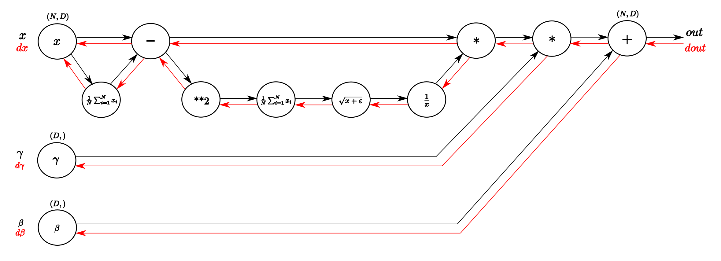
Structuring the CUDA Implementation

Following the structure suggested by the assignment documentation, we will implement the backward pass using two separate kernels. This is a common design pattern that can improve code modularity.

1. ker_ln_bw_dgamma_dbetta: This kernel will compute the gradients for the learnable parameters, $\nabla \gamma$ and $\nabla \beta$. Since both require a reduction over the same dimension, they can be computed efficiently together.
2. ker_ln_bw_dinp: This kernel will compute the more complex gradient for the input, $\nabla x$.

Kernel 1: Gradients for Scale ($\gamma$) and Bias ($\beta$)

Let's focus on ker_ln_bw_dgamma_dbetta. The task is to compute $\nabla {\gamma }_i={\sum }_j\nabla y_j{\hat{x}}_j$ and $\nabla {\beta }_i={\sum }_j\nabla y_j$. Each thread block will be responsible for computing the final gradient for a slice of the $\gamma$ and $\beta$ vectors.

The algorithmic steps, as outlined in the documentation, follow a classic parallel reduction pattern using shared memory and warp-level primitives.

The use of g.shfl_down is a key optimization. As you learned in Module 6, warp shuffle instructions allow threads within a warp to exchange data directly without going through shared memory, which is extremely fast.

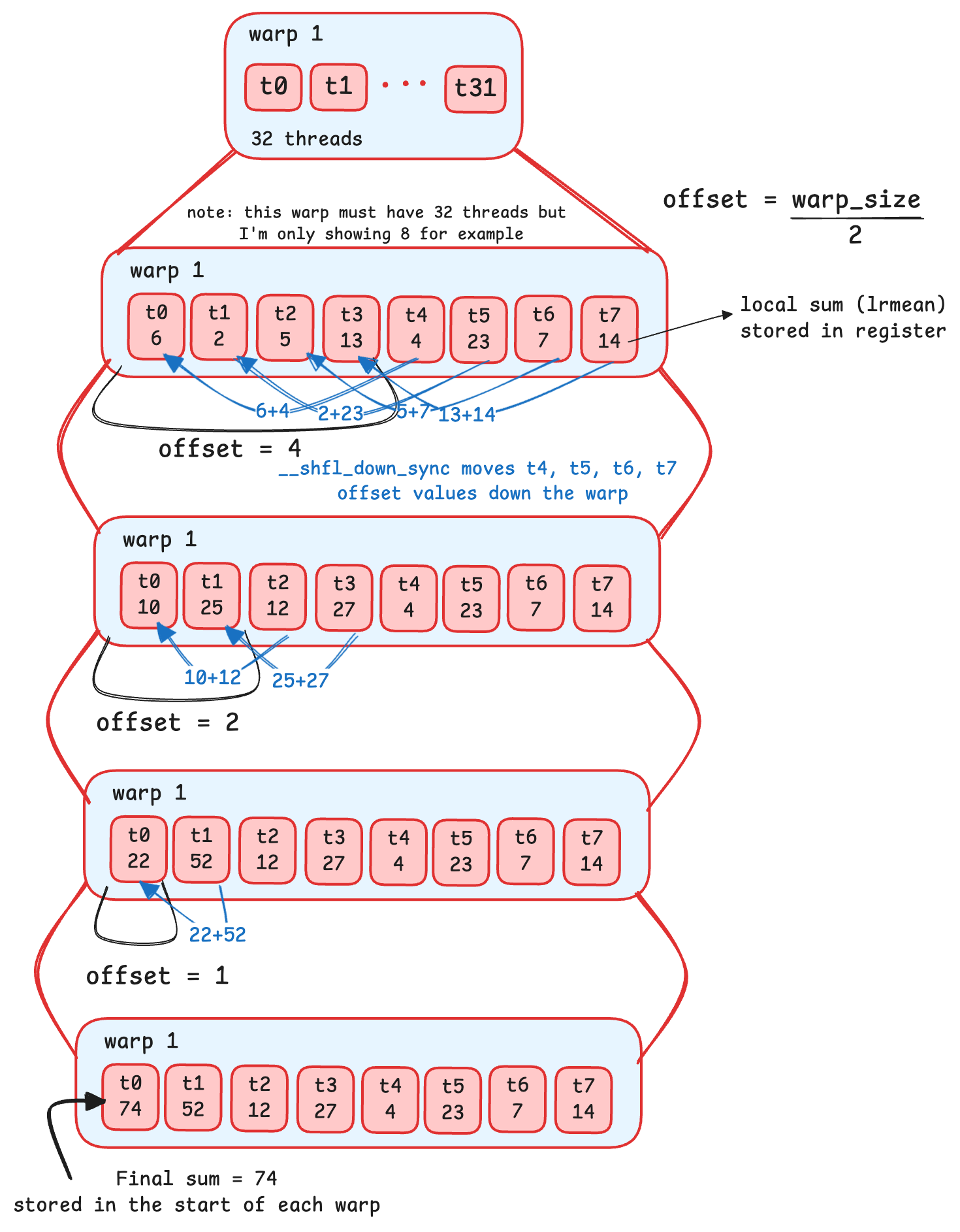
The overall process for this kernel within a single thread block would be:

1. Load Data: Each thread loads its share of out_grad, inp, means, and vars.
2. Partial Sums: Each thread computes a partial sum for $\nabla \gamma$ and $\nabla \beta$ over the elements it's responsible for.
3. Shared Memory Store: Threads store their partial sums into shared memory arrays.
4. Intra-Block Reduction: A parallel reduction is performed on the shared memory arrays. This is often done in two stages:
   • First, a reduction within each warp using __shfl_down_sync.
   • Then, one thread per warp writes its warp's sum to shared memory, and a final reduction across the warp results is performed.
5. Write Output: The thread with the final sum (e.g., threadIdx.x == 0) writes the result to global memory for gamma_grad and betta_grad.

Kernel 2: Gradient for Input ($x$)

Now, let's tackle ker_ln_bw_dinp. The goal is to compute $\nabla x_i$ for each input element. The formula depends on the two sums, $S_1={\sum }_j\nabla y_j{\gamma }_j$ and $S_2={\sum }_j(\nabla y_j{\gamma }_j){\hat{x}}_j$.

The strategy here is analogous to the serial C code: first, compute the reductions, and then use the results to compute the final gradient.

The blockReduce mentioned here would be a function that implements the shared-memory-based parallel reduction you built in Module 7. The steps for this kernel, processed by each thread block for its assigned row, are:

1. Parallel Reduction for $S_1$ and $S_2$:

   • Each thread computes a partial sum for $S_1$ and $S_2$ from the elements it loads. Remember to use vectorized loads (e.g., float4) for efficiency.
   • Threads collaborate using a shared memory reduction (blockReduce) to find the total sums for $S_1$ and $S_2$ for the entire block (i.e., for the entire feature dimension).
   • A __syncthreads() is critical here to ensure all threads have finished contributing to the reduction before any thread proceeds.

2. Compute Final Gradient:

   • After the __syncthreads(), the final sums $S_1$ and $S_2$ are available to all threads in the block (typically stored in shared memory).
   • Each thread can now compute its final $\nabla x_i$ value using the full formula, its local values ($\nabla y_i,{\gamma }_i,{\hat{x}}_i$), and the shared sums $S_1$ and $S_2$.
   • Each thread then writes its computed inp_grad value to global memory.

This two-phase approach (reduce, then calculate) is fundamental to parallelizing many machine learning operations.

Conclusion

In this lesson, you have translated the complex mathematics of the Layer Normalization backward pass into a concrete, high-performance parallel implementation strategy. This process is central to the work of a kernel optimization engineer.

Key Takeaways:

• The LayerNorm backward pass is dominated by parallel reduction operations.
• Rearranging analytical formulas can expose concurrency, such as the two independent summations needed for the $\nabla x$ calculation.
• A practical CUDA implementation can be split into multiple kernels (e.g., one for parameter gradients, one for input gradients) for modularity.
• Efficient reduction can be achieved using a combination of shared memory for inter-warp communication and warp shuffle instructions (__shfl_down_sync) for fast intra-warp communication.
• The overall algorithm follows a two-phase pattern: first, perform parallel reductions to compute necessary sums, synchronize, and then have each thread compute its final output using the shared reduction results.
• Techniques like vectorized memory access (e.g., float4) are crucial for maximizing memory bandwidth, just as they were in GEMM.

You have now implemented both the forward and backward passes for a fused Layer Normalization kernel. This is a significant milestone. In our next lesson, we will turn our attention to another essential component of the Transformer architecture: the Softmax function. We will start by analyzing its potential for numerical instability and implement a robust parallel version that addresses this issue.