Layer Normalization: Forward Pass with Parallel Reduction

The Mathematics of Layer Normalization

Before we can optimize, we must understand the computation itself. Layer Normalization's goal is to standardize the features for a given layer's input, which helps stabilize training. For each input feature vector (e.g., a row in a matrix), it calculates the mean and variance, then uses them to normalize the vector to have a mean of 0 and a variance of 1.

To ground our understanding, let's review the fundamental formulas.

As you've just read, the process for a single row $X_i$ with $n$ elements involves:

1. Mean Calculation: ${\mu }_i=\frac{1}{n}{\sum }_{j=1}^n{X}_{ij}$
2. Variance Calculation: ${\sigma }_i^2=\frac{1}{n}{\sum }_{j=1}^n(X_{ij}-{\mu }_i{)}^2$
3. Normalization: ${\hat{X}}_{ij}=\frac{X_{ij}-{\mu }_i}{\sqrt{{\sigma }_i^2+ϵ}}$

Notice that both the mean and variance calculations are reduction operations. This is the key to our parallel implementation.

From Math to Kernel: A Two-Pass Approach

A direct translation of the math suggests a multi-pass algorithm. For each row, you would:

1. Perform a parallel reduction to compute the sum, then divide to get the mean.
2. Perform a second parallel reduction, using the mean, to compute the sum of squared differences for the variance.
3. Loop over the elements a third time to apply the normalization.

This "two-pass" reduction strategy is a valid starting point. The parallel reductions for sum and variance can be efficiently implemented using the shared memory techniques you've already mastered.

While this shared memory approach works and is a massive improvement over a purely sequential calculation, it has two significant drawbacks:

1. Memory Bandwidth: The input data for a row is read from global memory at least twice: once for the mean calculation and a second time for the variance calculation.
2. Numerical Instability: The standard variance formula, often expressed as ${\sigma }^2=E[X^2]-(E[X]{)}^2$, can suffer from a problem called "catastrophic cancellation." If the mean is very large and the variance is very small, the subtraction of two large, nearly equal floating-point numbers can result in a massive loss of precision, sometimes even yielding a negative variance, which is mathematically impossible.

A More Robust Solution: The One-Pass Welford's Algorithm

To address both issues, we can use a more sophisticated method: Welford's online algorithm. This algorithm allows for the computation of both mean and variance in a single pass over the data and is numerically stable.

The standard Welford's algorithm updates three values as it iterates through data points $x_k$: a count count, a running mean mean, and an aggregate sum of squared differences from the mean, M2.

For a parallel implementation, the crucial insight is that we can derive a formula to combine the (count, mean, M2) tuples from two independent, parallel computations. If we have two chunks of data processed in parallel, resulting in tuples $(c_A,m_A,M_{2A})$ and $(c_B,m_B,M_{2B})$, we can combine them into a single, correct tuple for the combined dataset:

$c_{new}=c_A+c_B$
$\delta =m_B-m_A$
$m_{new}=m_A+\delta \cdot \frac{c_B}{c_{new}}$
$M_{2,new}=M_{2A}+M_{2B}+{\delta }^2\cdot \frac{c_A{c}_B}{c_{new}}$

This combination formula is the heart of a high-performance, parallel Welford reduction.

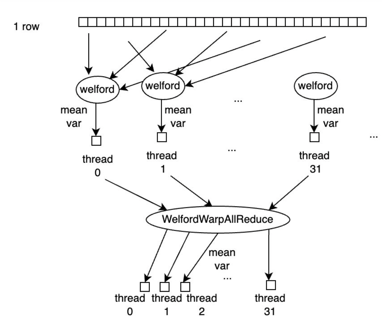
Let's now study an implementation that uses this exact technique.

Dissecting the Welford Kernel

Let's break down the layernorm_welford kernel into its logical stages. The overall strategy is to assign one thread block per row.

Stage 1: Per-Thread Partial Reduction

// Welford online algorithm
float mean = 0.0f, M2 = 0.0f;
int count = 0;
for (int i = tid; i < D; i += blockDim.x) {
    float val = x_row[i];
    count++;
    float delta = val - mean;
    mean += delta / count;
    M2 += delta * (val - mean);
}

This is the first part of the kernel. It uses a grid-stride loop, a pattern you're familiar with. Each thread processes a strided subset of the elements in the row. For each element it processes, it updates its own private count, mean, and M2 variables held in registers. This is the standard, sequential Welford's algorithm applied at the thread level. At the end of this loop, each thread has a correct (count, mean, M2) tuple for the elements it has processed.

Stage 2: Intra-Block Parallel Reduction

// Parallel Welford reduction across warp
for (int offset = 16; offset > 0; offset /= 2) {
    float other_mean = __shfl_down_sync(0xffffffff, mean, offset);
    float other_M2 = __shfl_down_sync(0xffffffff, M2, offset);
    int other_count = __shfl_down_sync(0xffffffff, count, offset);

    // Combine this thread's tuple with the 'other' thread's tuple
    int total = count + other_count;
    float delta = other_mean - mean;
    mean = (count * mean + other_count * other_mean) / total;
    M2 = M2 + other_M2 + delta * delta * count * other_count / total;
    count = total;
}

This is where the magic happens. This code performs the parallel reduction using warp shuffle instructions.

• __shfl_down_sync is used to get the (count, mean, M2) tuple from another thread in the warp.
• The lines that follow are a direct implementation of the parallel Welford combination formula we saw earlier.
• This loop reduces the tuples across the 32 threads of a warp. At the end, thread 0 (lane 0) of each warp holds the combined tuple for that entire warp.

(Note: The provided code snippet only shows reduction within a warp. A full implementation for blocks larger than 32 threads would require an additional step to combine the results from each warp, typically using shared memory, as you saw in the "Warp level Shuffle functions" section of the first blog post.)

Stage 3: Finalization and Normalization

// Broadcast the final result from lane 0
mean = __shfl_sync(0xffffffff, mean, 0);
float var = __shfl_sync(0xffffffff, M2, 0) / D;
float inv_std = rsqrtf(var + eps);

// Apply the normalization in a final fused pass
for (int i = tid; i < D; i += blockDim.x) {
    y_row[i] = (x_row[i] - mean) * inv_std * gamma[i] + beta[i];
}

1. The __shfl_sync(..., 0) instruction acts as a broadcast, ensuring all threads in the warp get the final mean and M2 values computed by lane 0.
2. inv_std is calculated.
3. Finally, another grid-stride loop is used. This time, the threads read their input elements again, apply the complete normalization formula using the now-known mean and inv_std, and write the final result to global memory. The gamma and beta terms are learnable affine parameters often included in LayerNorm, which we handle here.

This entire sequence—partial reduction, parallel combination, and final normalization—is fused into a single kernel, achieving high performance and numerical accuracy.

Conclusion

In this lesson, we have constructed a high-performance forward pass for Layer Normalization. You've seen how a deep understanding of the underlying mathematics, combined with advanced parallel primitives, allows us to create kernels that are both fast and robust.

Key Takeaways:

• The Layer Normalization forward pass is a fused operation combining parallel reduction with element-wise computation.
• A naive two-pass algorithm is simple to conceptualize but suffers from poor memory bandwidth usage and potential numerical instability.
• Welford's algorithm provides a numerically stable method to compute mean and variance in a single pass.
• Welford's algorithm can be parallelized by using a specific formula to combine the partial (count, mean, M2) tuples from different threads.
• An efficient implementation strategy uses one block per row, with each thread computing a partial result via a grid-stride loop, followed by an intra-block reduction using warp shuffles to produce the final mean and variance.

In our next lesson, we will tackle the other half of this operation: implementing the backward pass for Layer Normalization. This will require us to derive the gradients and implement an even more intricate kernel, further building on your growing expertise in writing high-performance code for AI.