Understanding Overfitting and Underfitting with Learning Curves

What are Learning Curves? A Visual Diagnostic

At its core, a learning curve is a plot that shows a model's performance as a function of experience or data. This "performance" is typically an error metric (like Mean Squared Error) or a score (like accuracy), while "experience" can be measured in two common ways:

1. By Training Iterations (Epochs): We plot the training and validation error after each pass through the training data (each epoch). This is useful for understanding the training dynamics of a single model.
2. By Training Set Size: We plot the performance as the model is trained on incrementally larger subsets of the data. This is the more formal definition and helps us understand if gathering more data would be beneficial.

Let's start with the first type, as it provides a direct, intuitive picture of the learning process. The following video offers an excellent analogy to build your intuition on how to interpret these plots.

As the video explains, we need to look at two curves simultaneously:

• Training Error/Loss: The error of the model on the same data it was trained on.
• Validation Error/Loss: The error of the model on a hold-out set of data it has not seen during training.

The relationship between these two curves is what allows us to diagnose the model's health.

Let's examine the three classic patterns you'll encounter.

1. Underfitting (High Bias): The top plot shows a model that is struggling. Both the training and validation errors are high and have flattened out. The model isn't even capable of fitting the training data well, so it certainly can't generalize. It's too simple for the task.

2. Overfitting (High Variance): The middle plot is a classic case of overfitting. The training error becomes very low—the model has effectively "memorized" the training set. However, the validation error starts to decrease but then begins to rise again (or stays high). This growing gap between the curves signals that the model is learning noise and details specific to the training set that do not generalize.

3. Good Fit: The bottom plot shows what we aim for. Both training and validation errors decrease and converge to a low value. There is a minimal gap between the two curves, indicating that the model has learned the general patterns in the data without memorizing its noise.

This second image highlights a key strategy for dealing with overfitting that is directly visible from this type of learning curve.

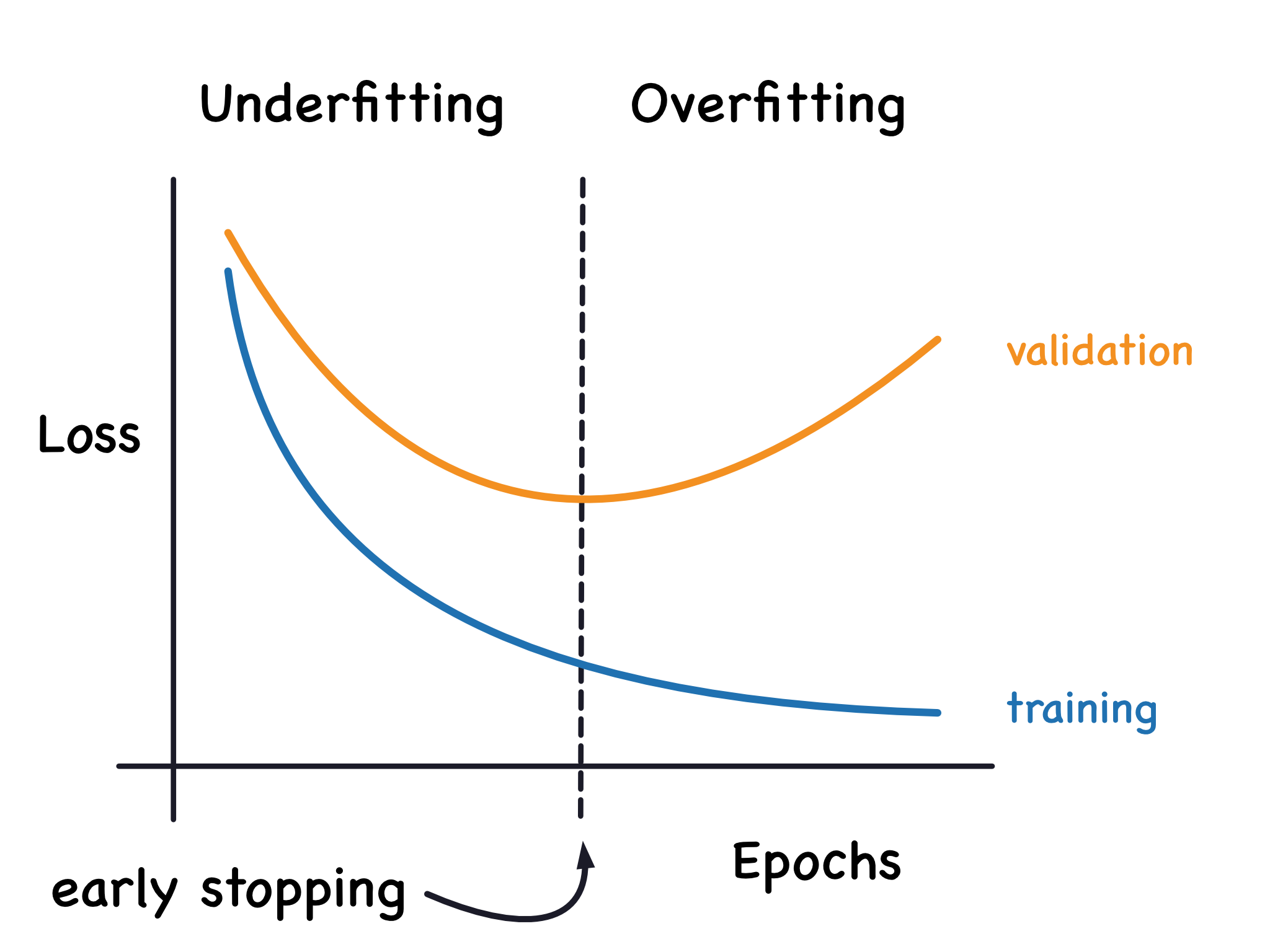
When a model starts to overfit, we can simply stop the training process at the point where the validation error is at its minimum. This technique is aptly named early stopping and is a very common and effective form of regularization.

Learning Curves vs. Training Data Size

Now let's turn to the more formal definition of a learning curve, which plots performance against the number of training samples used. This tool answers a critical question: "Will my model improve if I collect more data?"

The scikit-learn documentation provides a concise explanation and shows how these curves are generated.

Let's consolidate what these curves tell us:

• Diagnosing High Bias (Underfitting): If a model is too simple, its performance will be poor, regardless of how much data you give it. The learning curve will show the training and validation errors converging to a high value (or, if plotting accuracy, a low value). The curves meet, but they meet at an unacceptable performance level. In this case, adding more data is futile; you need a more complex model.

• Diagnosing High Variance (Overfitting): If a model is too complex, it will perform very well on small amounts of data because it can easily memorize them. As the training set size increases, the training error will rise (it's harder to memorize more data) and the validation error will fall (the model is forced to learn more general patterns). The key sign is a large gap between the training and validation error. The fact that the validation error is still decreasing as data is added suggests that collecting more data is a viable strategy to improve generalization.

To see these patterns analyzed in detail, the following article provides a step-by-step interpretation of learning curves for a good fit, an overfit model, and an underfit model.

Clarification: Learning Curves vs. Validation Curves

You may notice a similarity between these plots and the error plots from our previous lesson, which showed error as a function of model complexity. It's important to distinguish between these two diagnostic tools, as they answer different questions.

• Learning Curve: Plots performance vs. training set size. It answers the question: "Will more data help?"
• Validation Curve: Plots performance vs. a model hyperparameter (e.g., the degree of a polynomial, the C parameter in an SVM). It answers the question: "How does this specific measure of model complexity affect performance?"

A validation curve is what you would use to find the "sweet spot" in the bias-variance tradeoff for a particular hyperparameter. A learning curve tells you whether you are limited by your model's intrinsic bias or by the amount of data you have. The scikit-learn documentation, which you reviewed a moment ago, also has a section on validation curves that makes this distinction clear.

Conclusion

In this lesson, we have bridged the gap between the theory of the bias-variance tradeoff and its practical diagnosis. Learning curves are an indispensable tool in the machine learning practitioner's toolkit.

Here are the key takeaways:

• Learning curves visualize the relationship between training error and validation error as training progresses or as the training set size increases.
• Underfitting (high bias) is identified when both training and validation errors are high and converge. This suggests the model is too simple and adding more data will not help.
• Overfitting (high variance) is identified by a large and persistent gap between a low training error and a high validation error. This suggests the model is too complex and may benefit from more data or regularization (like early stopping).
• A well-fit model shows both training and validation errors converging at a low value with a minimal gap between them.

You now understand the fundamental problems of underfitting and overfitting, their theoretical basis in bias and variance, and how to spot them using learning curves. The next logical step is to start building models ourselves. In the upcoming lesson, we will get our hands dirty by setting up a standard machine learning project environment with essential Python libraries like NumPy, pandas, and scikit-learn. This will lay the groundwork for implementing, training, and evaluating our very first models.