Bias-Variance Tradeoff: Impact on Model Generalization

The Anatomy of Error: Bias and Variance

At a high level, the total error of a machine learning model on unseen data can be thought of as stemming from three sources:

1. Bias: This represents the error from erroneous assumptions in the learning algorithm. High bias can cause an algorithm to miss the relevant relations between features and target outputs. We can think of it as a systematic error or the model's inherent inflexibility. A model with high bias is underfitting the data.
2. Variance: This represents the error from sensitivity to small fluctuations in the training set. High variance can cause an algorithm to model the random noise in the training data, rather than the intended outputs. It reflects the model's instability. A model with high variance is overfitting the data.
3. Irreducible Error: This error is due to the inherent noise in the data itself. No matter how good our model is, we cannot reduce this error. It represents a lower bound on the error for any model.

The "tradeoff" comes from the fact that, for a given model, decreasing one of these error components often leads to an increase in the other.

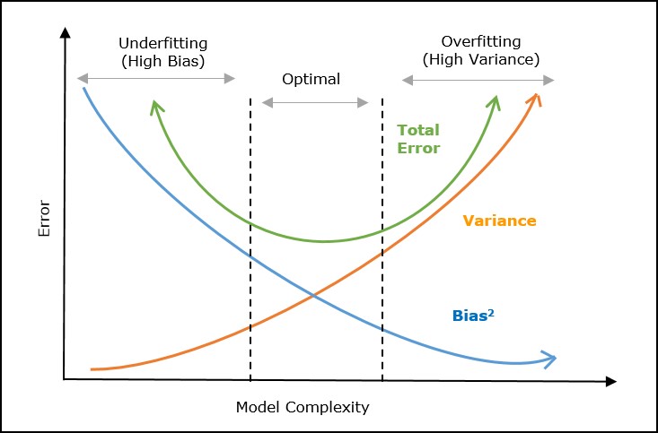
To build an initial intuition, let's explore an interactive article that visualizes these concepts.

The Mathematical Foundation of the Tradeoff

Your strong mathematical background will be an asset here as we formalize these ideas. The bias-variance decomposition provides a precise mathematical breakdown of the expected error. We will focus on the Mean Squared Error (MSE) for a regression problem, as it allows for a clean decomposition.

Professor Yaser Abu-Mostafa from Caltech provides one of the clearest derivations of this concept. His explanation hinges on the idea of an "average hypothesis," which is a conceptual tool to understand the model's behavior across many different training datasets.

Let's summarize the key mathematical result. If our true model is $y=f(x)+ϵ$, where $ϵ$ is noise with mean 0 and variance ${\sigma }^2$, then the expected prediction error of our learned model $\hat{f}(x)$ at a point $x_0$ is:

Let's break down each term:

• Bias²: The squared difference between the average prediction of our model (across all possible training sets) and the true function value. This measures how far off the model's average prediction is from the truth. A simple model, like a linear one trying to fit a curve, will have high bias.
• Variance: The variance of the model's predictions for a given point $x_0$. This measures how much the model's prediction $\hat{f}(x_0)$ "jiggles" or varies as we use different training sets. A complex model that fits noise will have high variance.
• Irreducible Error (${\sigma }^2$): The variance of the noise term $ϵ$. This is the lower bound of error that we can never overcome, regardless of the model we choose.

For a more condensed, text-based walkthrough of this derivation, you can refer to the following lecture notes.

Visualizing the Tradeoff with a Concrete Example

Theory is best understood through application. The Stanford Statistical Learning course provides excellent visualizations of the tradeoff using simulated data. The video shows how the test error curve is formed by the sum of the bias-squared and variance curves as model flexibility changes.

The key insight is that as we make our model more flexible (e.g., use a higher-degree polynomial, a more complex spline, or a deeper decision tree), the bias consistently goes down because the model has more power to approximate the true function. However, the variance goes up because the model has more freedom to fit the random noise specific to the training set. Our goal is to find the "sweet spot" of complexity that minimizes their sum.

Implications for Generalization and Model Development

Understanding the bias-variance tradeoff has direct, practical implications for building models that generalize well. When you evaluate your model on the validation set and find that the error is high, you can use this framework to diagnose the problem and decide on a course of action.

• If your model suffers from high bias (underfitting):

  • Symptom: The model performs poorly on both the training set and the validation set. It's too simple to capture the underlying patterns.
  • Remedies:
    • Increase model complexity (e.g., switch from linear regression to a polynomial or a tree-based model).
    • Engineer new features that might have a stronger relationship with the target.
    • Reduce regularization, which penalizes complexity.

• If your model suffers from high variance (overfitting):

  • Symptom: The model performs extremely well on the training set but poorly on the validation set. It has memorized the training data, including its noise.
  • Remedies:
    • Decrease model complexity (e.g., use a simpler model, reduce the depth of a decision tree).
    • Gather more training data. More data helps the model learn the true signal and ignore the noise.
    • Increase regularization to penalize large model weights and discourage overly complex solutions.

This diagnostic process is a fundamental skill in applied machine learning. By analyzing your model's performance, you are essentially trying to locate where it sits on the U-shaped error curve and then taking steps to move it toward the minimum.

Conclusion

In this lesson, we have moved from simply measuring generalization error to understanding its constituent parts. The bias-variance tradeoff provides a theoretical lens through which we can analyze and improve our models.

Here are the essential takeaways:

• A model's expected error on unseen data can be decomposed into Bias², Variance, and Irreducible Error.
• Bias is a systematic error caused by a model's simplifying assumptions (leading to underfitting).
• Variance is an error caused by a model's excessive sensitivity to the training data (leading to overfitting).
• There is an inherent tradeoff: increasing model complexity typically reduces bias but increases variance. The goal of model selection is to find the optimal complexity that minimizes the total error.
• This framework provides a roadmap for model improvement: diagnosing high error as either a bias or variance problem suggests specific remedies.

We've now established what the problems of underfitting and overfitting are in terms of bias and variance. But how do we spot them in a real project? In our next lesson, we will learn how to diagnose these issues practically by plotting and interpreting learning curves, which show how training and validation errors change as the amount of training data increases.