Visualizing Data Distributions with Histograms and Box Plots

1. Histograms: Visualizing the Shape of Your Data

Imagine you have 100 measurements of nanoparticle diameters from a synthesis batch. Simply listing the numbers or calculating a mean and standard deviation doesn't reveal the full story. Is the distribution of sizes symmetric? Are there two distinct populations of sizes (bimodal)? Is the data skewed towards larger or smaller particles?

A histogram answers these questions by grouping data into "bins" and plotting the frequency of measurements in each bin.

To get a clear, intuitive understanding of how histograms work, please watch the following video.

The Critical Importance of Bin Width

As the video hinted, the most important decision you make when creating a histogram is choosing the bin width. An inappropriate bin width can obscure important features or even create misleading patterns.

• Too wide: Oversimplifies the distribution, hiding features like multiple peaks.
• Too narrow: Creates a noisy, jagged plot where it's hard to see the underlying trend.

Let's continue with the same video to see a demonstration of this effect.

The key takeaway is that you should always experiment with different bin widths to ensure the visualization accurately reflects your data's structure.

2. Box Plots: A Five-Number Summary

While histograms are great for seeing the detailed shape of a single distribution, box plots (or box-and-whisker plots) provide a more condensed summary. They are exceptionally useful for comparing multiple datasets at a glance, a common task when evaluating different experimental conditions or analytical methods.

A box plot is constructed from five key statistical values:

1. Minimum: The lowest value in the dataset (excluding outliers).
2. First Quartile (Q1): The 25th percentile. 25% of the data falls below this value.
3. Median (Q2): The 50th percentile, which we've previously discussed as a measure of central tendency.
4. Third Quartile (Q3): The 75th percentile. 75% of the data falls below this value.
5. Maximum: The highest value in the dataset (excluding outliers).

The Interquartile Range (IQR = Q3 - Q1) is a robust measure of spread, similar to the standard deviation we covered in the last lesson. Because it focuses on the middle 50% of the data, it is less affected by extreme values.

Constructing and Interpreting a Box Plot

The following video provides a step-by-step guide on how to calculate the necessary values and construct a box plot from a raw dataset.

As the video explained, a key function of box plots is to flag potential outliers. The standard rule is to define the "whiskers" of the plot as extending to the furthest data points that are within 1.5 times the IQR from the edges of the box (Q1 and Q3). Any data point that falls outside of this range is plotted as an individual point and considered a potential outlier. We will explore this in more detail in the next lesson.

3. Histograms vs. Box Plots: Choosing the Right Tool

So, when should you use a histogram, and when is a box plot more appropriate? They are complementary tools that answer different questions.

• Use a histogram when you want to understand the detailed shape, skewness, and modality (number of peaks) of a single dataset.
• Use a box plot when you want to concisely summarize a dataset or, more importantly, compare the distributions of several datasets side-by-side.

The image below shows how three different datasets are represented by both histograms and box plots.

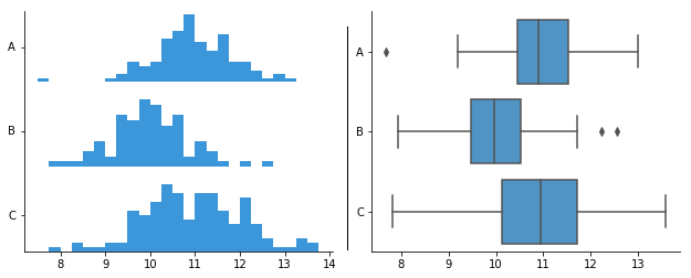
Notice how the box plots make it very easy to compare the medians (the line in the box), the spread (the height of the box), and the presence of outliers across the three groups. Trying to overlay the three histograms would be visually cluttered and much harder to interpret.

For further reading on the roles and interpretation of these plots, you can review the following text.

4. Practice Problem

Let's apply these concepts. In your lab, you are comparing two purification methods for a synthesized compound. You run five replicates for each method and measure the final purity (%).

• Method A (% Purity): 98.5, 98.7, 99.0, 99.1, 99.2
• Method B (% Purity): 95.2, 98.4, 98.6, 98.8, 100.0

For Method B, calculate the five-number summary and the IQR. Would any points be flagged as outliers by the 1.5xIQR rule? Based on the summary statistics, how might a box plot for Method B differ from a box plot for Method A?

Conclusion

You have now learned how to construct and interpret two of the most fundamental data visualization tools in science and statistics.

Key Takeaways:

• Histograms are excellent for visualizing the detailed shape, center, and spread of a single continuous variable. The choice of bin width is critical for accurate interpretation.
• Box plots provide a compact summary based on five key numbers (min, Q1, median, Q3, max). They are ideal for comparing distributions across multiple groups and flagging potential outliers.
• The Interquartile Range (IQR) is a robust measure of spread used in box plots.

In this lesson, we introduced the concept of identifying outliers using the 1.5xIQR rule. In our next lesson, we will dedicate our full attention to this topic: Identify potential outliers in analytical data using box plots and the IQR rule. We will formalize this process and then learn a statistical test to help confirm if an apparent outlier should be retained or rejected.