Identifying Outliers with Box Plots and the IQR

1. What is an Outlier and Why Does It Matter?

In any experimental work, especially in analytical chemistry, we occasionally encounter measurements that seem out of place. Imagine you're running a series of standards on an atomic absorption spectrometer. If one reading is drastically different from the others for the same standard, you instinctively check for an issue—a dilution error, a bubble in the sample line, or a data transcription mistake.

Statistically, an outlier is an observation that appears inconsistent with other observations in the dataset. It's a data point that has a low probability of originating from the same statistical distribution as the rest of the data. To understand the formal definition and its importance in a regulated environment, please read the introductory section of the following article from Pharmaceutical Technology.

As the article states, an outlier isn't just a nuisance; it can be a valuable signal that points to a shift in your process, a problem with your measurement system, or an error in your procedure. Identifying potential outliers is the first step toward a root cause investigation.

2. The IQR Rule for Identifying Potential Outliers

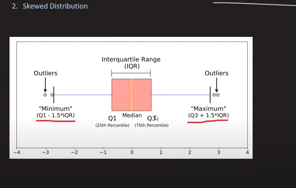
The box plot gives us a visual hint about outliers, but we need a consistent numerical rule to identify them. The most common method, which we touched on in the last lesson, is the 1.5 x IQR rule.

This rule establishes invisible "fences" on either side of our data's central bulk. Any data point that falls outside these fences is flagged as a potential outlier.

Here are the components:

• Interquartile Range (IQR): As a reminder, this is the range of the middle 50% of your data, calculated as IQR = Q3 - Q1.
• Lower Fence: The lower boundary for our data. Any point below this is a potential outlier.
  $\text{Lower Fence}=Q1-(1.5\times \text{IQR})$
• Upper Fence: The upper boundary. Any point above this is a potential outlier.
  $\text{Upper Fence}=Q3+(1.5\times \text{IQR})$

The image below provides a clear visual representation of this concept.

Now, let's watch a short video that walks through a concrete calculation.

This method is widely used because it's non-parametric, meaning it doesn't assume your data follows a specific distribution (like the normal distribution). Since the rule is based on quartiles and the median, it is "robust" and not heavily influenced by the very outliers it is designed to find.

3. A Step-by-Step Example

Let's solidify this with a practical example relevant to your work.

Suppose you are measuring the concentration of lead (in ppb) in a water sample using AAS. You take 10 replicate measurements to assess the method's precision.

Data (ppb): 15.2, 15.4, 15.1, 15.5, 15.3, 16.9, 15.2, 15.4, 15.6, 15.3

Does the value 16.9 qualify as a potential outlier? Let's apply the 1.5 x IQR rule.

1. Order the data:
   15.1, 15.2, 15.2, 15.3, 15.3, 15.4, 15.4, 15.5, 15.6, 16.9

2. Find the Median (Q2):
   With 10 data points, the median is the average of the 5th and 6th values:
   $\text{Median}=\frac{15.3+15.4}{2}=15.35$

3. Find the Quartiles (Q1 and Q3):

   • Lower half of data: 15.1, 15.2, 15.2, 15.3, 15.3. The median of this half is Q1 = 15.2.
   • Upper half of data: 15.4, 15.4, 15.5, 15.6, 16.9. The median of this half is Q3 = 15.5.

4. Calculate the IQR:
   $\text{IQR}=Q3-Q1=15.5-15.2=0.3$

5. Calculate the Fences:

   • Lower Fence: $Q1-(1.5\times \text{IQR})=15.2-(1.5\times 0.3)=15.2-0.45=14.75$
   • Upper Fence: $Q3+(1.5\times \text{IQR})=15.5+(1.5\times 0.3)=15.5+0.45=15.95$

6. Identify Outliers:
   The range of acceptable data is [14.75, 15.95]. Our dataset includes the value 16.9, which is above the upper fence. Therefore, 16.9 is flagged as a potential outlier.

On a modified box plot, the upper whisker would extend only to 15.6 (the largest value still within the fence), and 16.9 would be plotted as a separate point.

4. Practice and Interpretation

Now it's your turn. In a lab developing a new paper-based microfluidic device for glucose detection, you run 15 tests on a standard solution. The color intensity readings are recorded.

Data (Intensity Units):
6, 9, 15, 15, 18, 22, 5, 27, 32, 33, 10, 14, 16, 8, 40

1. Calculate the IQR.
2. Determine the lower and upper outlier fences.
3. Are there any outliers in this dataset?

This practice problem highlights a key point: our intuition can sometimes be misleading. A formal rule provides an objective criterion for flagging data. However, remember the guidance from the Pharmaceutical Technology article: flagging a point is not justification for removing it. It is a signal to investigate. Was there a contamination issue with the sample that gave the 40 reading? Was the device improperly fabricated? Or is it simply a legitimate, though high, result from a skewed data distribution?

Conclusion

In this lesson, you have learned a standard and robust method for flagging potential outliers in your experimental data. This is a crucial skill for data quality assessment in any analytical field.

Key Takeaways:

• An outlier is a data point that appears inconsistent with the rest of the data and may signal an error or an important process deviation.
• The 1.5 x IQR rule provides a quantitative method for identifying potential outliers by defining lower and upper "fences."
• The formulas for the fences are: Lower Fence = Q1 - (1.5 x IQR) and Upper Fence = Q3 + (1.5 x IQR).
• Identifying a potential outlier is the beginning of an investigation, not an automatic justification for data removal.

The IQR rule is an excellent screening tool. However, it does not provide a statistical probability that a point is a true outlier. In our next lesson, we will advance to a formal statistical test. We will learn how to apply Grubb's test to statistically confirm and handle outliers in a dataset, which will give you a more powerful tool for making decisions, especially when you can assume your data is approximately normally distributed.