Pipelining and Latency

1. Distinguishing Latency from Throughput

Before we dive into the numbers, it's essential to have a solid intuitive grasp of the difference between latency and throughput. They are two distinct measures of performance that are often traded against one another.

A great way to visualize this is to think of a tunnel.

As the article explains:

• Latency is the total time it takes for one "car" (one piece of data) to get from the entrance to the exit of the "tunnel" (your circuit). It's measured in units of time, like nanoseconds.
• Throughput is the rate at which cars exit the tunnel. It's measured as operations per unit of time, like millions of operations per second.

Pipelining is like adding more lanes to the tunnel. It doesn't make any single car travel faster (in fact, as we'll see, it can slow it down slightly), but it allows many more cars to pass through over the same period.

2. Calculating Pipelined Latency

In the last lesson, we saw that pipelining involves breaking a computation into $K$ stages, separated by registers. A piece of data must pass through one register per clock cycle to advance to the next stage.

Therefore, the total time it takes for one input to produce an output—the latency—is determined by the number of stages and the clock period.

Latency = K stages × Clock Period ($T_{clk}$)

This means a 3-stage pipeline will take 3 clock cycles for data to traverse, a 5-stage pipeline will take 5, and so on.

The following video from MIT OpenCourseWare formalizes this relationship and provides a clear example.

3. Why Latency Increases with Pipelining

As the video highlights, the latency of a pipelined system is often slightly longer than the original unpipelined combinational delay. This might seem counterintuitive, but there are two main reasons for it.

1. Register Overhead: The clock period ($T_{clk}$) isn't just the logic delay. It must also account for the register's own timing characteristics: its clock-to-q delay ($t_{C-Q}$) and setup time ($t_{su}$). So, $T_{clk}\ge t_{\text{logic}}+t_{C-Q}+t_{su}$. Each pipeline stage introduces this small but non-zero overhead.

2. Unbalanced Stages: It is often impossible to divide the logic into perfectly balanced stages. The clock period for the entire pipeline must be long enough for the single slowest stage. The other, faster stages will sit idle for the remainder of the clock cycle, adding to the total latency.

Let's look at a concrete example.

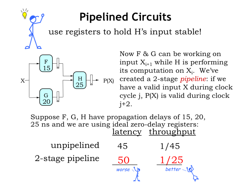
In the example shown in the "Pipelined Circuits" image:

• Unpipelined System:
  • Total propagation delay ($t_{PD}$) = 45 ns.
  • Latency = 45 ns.
  • Throughput = 1 / 45 ns ≈ 22 M ops/sec.
• Pipelined System:
  • The logic is split into two stages. The slowest stage (H) has a delay of 25 ns.
  • The clock period must be at least 25 ns (ignoring register overhead for simplicity).
  • Latency = 2 stages × 25 ns/stage = 50 ns.
  • Throughput = 1 / 25 ns = 40 M ops/sec.

Notice that the latency for a single operation increased from 45 ns to 50 ns. This is the cost paid for nearly doubling the throughput.

4. The Design Choice: Throughput vs. Latency

Pipelining is not a "free lunch." It is a deliberate architectural choice that prioritizes throughput at the expense of latency.

• High-Throughput Applications: For tasks involving streams of data like video encoding, network packet processing, or graphics rendering, throughput is king. The initial delay (latency) to process the first piece of data is insignificant compared to the need to process billions of subsequent data points as fast as possible. Pipelining is the go-to technique here.

• Low-Latency Applications: In other cases, the absolute time-to-result for a single operation is the most critical factor. Consider a control system reacting to a sensor input. Here, you might choose to use less (or no) pipelining to minimize the reaction time.

This article discusses when you might prioritize a low-latency design.

As a designer, you must analyze the requirements of your application to decide where on the throughput-latency spectrum your design should lie.

Conclusion

In this lesson, we've taken a closer look at the impact of pipelining on latency. While it's a fantastic tool for improving throughput, that benefit comes at the cost of increased latency for any individual operation.

Key Takeaways:

• Latency is the total time for a single piece of data to travel from input to output.
• Pipelining increases latency. The latency of a $K$-stage pipeline is $K\times T_{clk}$.
• This increased latency is due to the cumulative delay of clocking data through multiple registers and the fact that the clock period is set by the slowest stage.
• The decision to pipeline is a fundamental design trade-off. You sacrifice single-operation speed (latency) to gain a higher overall data processing rate (throughput).

In our next lesson, we will begin to piece together the concepts we've learned—combinational logic, sequential elements, and pipelining—to understand the structure of a simple processor datapath. We'll see how components like the ALU and register file are organized and how pipelining enables them to execute instructions efficiently.