Profiling-Driven Optimization and Verification

1. The Optimization Cycle

Effective optimization is a science, not an art. It follows a deliberate, iterative cycle. Guesswork leads to "premature optimization," which adds complexity for little or no real-world benefit. The cycle is simple:

1. Measure: Use benchmarks to establish a quantitative baseline for your system's performance. You can't improve what you don't measure.
2. Profile: Run those same benchmarks while collecting performance data (CPU, memory profiles). Analyze this data to identify the biggest bottlenecks, or "hotspots."
3. Optimize: Write code to fix the single most significant hotspot you identified. Don't try to fix everything at once.
4. Verify: Rerun the benchmarks and compare the new results against your baseline to prove that your change had the desired effect. If it did, this new result becomes your baseline for the next cycle.

This iterative process is fundamental to building high-performance systems.

2. Step 1: Establish a Baseline

First, we need our baseline. In a previous lesson, you created benchmarks for producer throughput and latency. We will use these to measure our broker's performance before making any changes.

To make comparison easy, it's best practice to save the benchmark output to a file. Navigate to your project's root directory and run your benchmarks.

# The -count=10 flag runs the benchmark suite 10 times to get a stable average.
# The `>` operator redirects the output to a file named `before.txt`.
go test -bench . -benchmem -count=10 ./... > before.txt

Note: Ensure your benchmark name (BenchmarkProducerThroughput, for example) is specific enough that you're only benchmarking the relevant part of the broker. The ./... ensures it finds the test package.

After this command completes, you will have a before.txt file containing results that look something like this:

BenchmarkProducerThroughput-16    1000    125368 ns/op    18952 B/op    215 allocs/op
... (9 more lines) ...

This file is our baseline. Any changes we make will be measured against these numbers.

3. Step 2: Profile to Identify a Hotspot

Now, let's find out where the program is spending its time and memory. We'll re-run the benchmark, but this time we'll enable CPU and memory profiling.

go test -bench . -benchmem -count=10 -cpuprofile cpu.prof -memprofile mem.prof ./...

This command does the same benchmarking as before, but it also generates two new files: cpu.prof and mem.prof. These contain the raw data for our analysis.

We will use the interactive web UI of pprof to explore the CPU profile.

go tool pprof -http=:8080 cpu.prof

This will open a new tab in your browser.

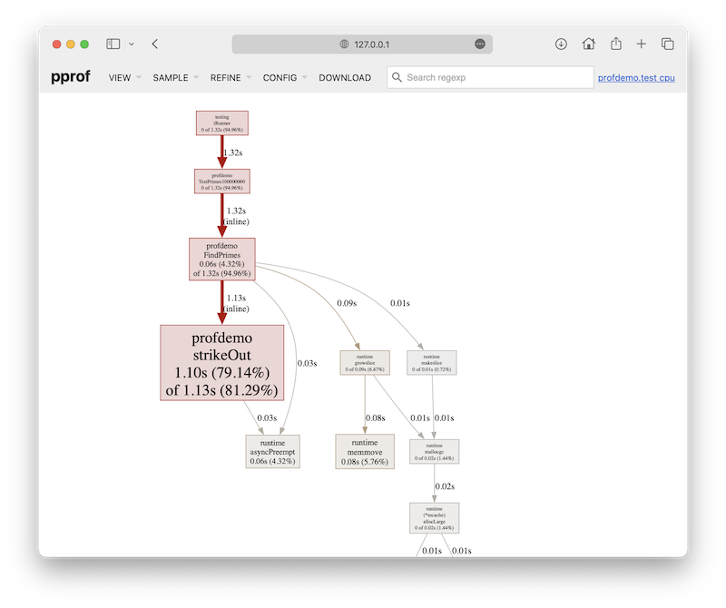
In the UI, navigate to the Flame Graph view from the "VIEW" dropdown. Flame graphs are often easier to read for identifying hotspots. Look for wide plateaus in the graph that originate from your benchmark function. These represent functions where significant CPU time is being spent.

Let's assume your analysis points to a function responsible for parsing incoming messages on the TCP connection. A common initial implementation might look something like this, where you use a general-purpose but inefficient function to extract a fixed-size field. This is inspired by a real optimization shown in Peter Bourgon's talk.

Hypothetical Hotspot:
Imagine in your TCP connection handler, you have code to parse a message frame that looks like [26-byte-ULID][payload]. A naive implementation might be:

// In your connection handler...
func parseMessage(data []byte) (ulid string, payload []byte) {
    // This is inefficient: it allocates a new slice for parts,
    // and scans for whitespace which we don't even have.
    parts := bytes.Fields(data) 
    if len(parts) > 0 {
        // Assume the first "field" is the ULID
        return string(parts[0]), bytes.Join(parts[1:], []byte(" "))
    }
    return "", data
}

Your pprof graph would likely show a large amount of time spent inside bytes.Fields. This is our target.

4. Step 3: Apply a Targeted Optimization

Once you've identified a hotspot, the goal is to replace it with a more efficient implementation. The key is to use your knowledge of the system to make a more specific, optimized choice.

In our hypothetical example, we know the ULID is always 26 bytes long. We don't need a general-purpose function like bytes.Fields. We can perform a direct slice operation, which is much faster and performs zero allocations.

The Optimization:
Replace the naive parseMessage with this optimized version:

const ulidLength = 26

func parseMessage(data []byte) (ulid string, payload []byte) {
    if len(data) < ulidLength {
        return "", data // Not a valid message
    }
    
    // This is a direct slice operation. It's extremely fast and
    // doesn't allocate new memory for the underlying data.
    ulidBytes := data[:ulidLength]
    payload = data[ulidLength:]
    
    return string(ulidBytes), payload
}

This change is small, localized, and directly attacks the bottleneck we identified with pprof.

5. Step 4: Verify the Impact

You've made a change, but did it work? And how much did it help? We must return to our benchmarks to answer these questions.

First, install benchstat, a tool from the Go team designed for comparing benchmark results.

go install golang.org/x/perf/cmd/benchstat@latest

Now, run the same benchmark command as in Step 1, but save the output to a different file, after.txt.

# Make sure your code changes from Step 3 are saved!
go test -bench . -benchmem -count=10 ./... > after.txt

Finally, use benchstat to compare the before.txt and after.txt files.

benchstat before.txt after.txt

You will see a clean, statistical comparison of the results:

name                   old time/op    new time/op    delta
ProducerThroughput-16    125µs ± 2%      85µs ± 3%    -32.00%  (p=0.000 n=10)

name                   old alloc/op   new alloc/op   delta
ProducerThroughput-16    18.5kB ± 1%    12.1kB ± 2%    -34.59%  (p=0.000 n=10)

name                   old allocs/op  new allocs/op  delta
ProducerThroughput-16     215 ± 0%       150 ± 1%    -30.23%  (p=0.000 n=10)

Interpreting the benchstat Output:

• delta: This is the most important column. A negative percentage means an improvement (less time, less memory).
• p=0.000: This is the p-value from a statistical test. A low value (e.g., < 0.05) indicates the change is statistically significant and not just random noise.
• ± 2%: This shows the variance in the benchmark runs.

In this example, our optimization yielded a ~32% reduction in CPU time, a ~34% reduction in memory usage, and a ~30% reduction in the number of allocations per operation. This is a clear, measurable win. We have successfully completed one full optimization cycle.

Conclusion

Congratulations! You have just performed a professional-grade performance optimization. You didn't guess; you measured, profiled, implemented a targeted fix, and verified the result. This disciplined cycle is the key to building and maintaining high-performance Go applications.

Key Takeaways:

• Don't Optimize Blindly: Always follow the "Measure, Profile, Optimize, Verify" cycle. Data, not intuition, should drive your optimization efforts.
• Use the Right Tools: go test -bench, pprof, and benchstat are the standard, powerful tools for this workflow in Go.
• Focus on Hotspots: The Pareto principle (80/20 rule) often applies to performance. Find the 20% of your code that's causing 80% of the load and focus your efforts there.
• Verify Everything: A change isn't an optimization until you have benchmark data that proves it.

Next Up

This lesson concludes our module on performance analysis and optimization. You now have the skills to diagnose and fix the most critical performance and correctness issues in a concurrent Go application.

In the final module of this course, Building the CLI and Deploying the System, we will shift our focus from the internal workings of the broker to its external interface and operation. We'll build a command-line tool to interact with our broker and then containerize the entire system for deployment. The performant, reliable core you've just hardened will serve as the engine for the complete system we're about to build.