Profiling CPU Hotspots with pprof

Hello again. In our last lesson, we instrumented our message broker with pprof's HTTP endpoints, effectively opening a window into its live operation. We now have the ability to collect performance data.

Today, we move from instrumentation to analysis. This lesson is dedicated to achieving the learning outcome: Use pprof to capture and analyze a CPU profile to identify performance hot spots. We will put our broker under a realistic load, capture a CPU profile, and learn the systematic process of reading the results to find the exact parts of our code that are consuming the most resources. This is one of the most critical skills for a systems programmer, as it replaces guesswork with data-driven diagnosis.

1. Capturing a Live CPU Profile

To get a meaningful profile, we need to analyze the application while it's doing work. Profiling an idle server is not very informative. We will use the producer benchmark we wrote previously to generate a sustained load and then capture a CPU profile during that load.

Here is the three-step process:

Start the Broker: In one terminal, navigate to your project directory and run the broker.
```
go run ./cmd/broker
```
You should see the log message indicating the broker is listening, as well as the observability server on port 6060.
Generate Load: In a second terminal, we will run our producer throughput benchmark. By using the -benchtime flag, we can run it for a fixed duration, which is perfect for creating sustained load. Let's run it for 30 seconds.
```
go test ./... -bench=BenchmarkProducerThroughput -benchtime=30s -v
```
You will see the benchmark start and run for approximately 30 seconds.
Capture the Profile: While the benchmark is running, open a third terminal. We'll use the go tool pprof command to connect to our broker's live endpoint and sample its CPU activity. We'll sample for 25 seconds to ensure we capture the activity during the peak load period.
```
go tool pprof -http=:8081 http://localhost:6060/debug/pprof/profile?seconds=25
```
After 25 seconds, this command will finish collecting data and automatically open a new tab in your web browser at http://localhost:8081. This is the interactive pprof web UI.

You now have a snapshot of where your broker spent its CPU cycles under load.

2. The Art of Analysis: Reading the Profile

The pprof UI can be intimidating at first, but its analysis follows a simple principle: find what took the most time and drill down.

2.1 The Big Picture: Graph vs. Flame Graph

The pprof UI offers several views (visualizations) of the same data. The two most important for an initial analysis are Graph and Flame Graph.

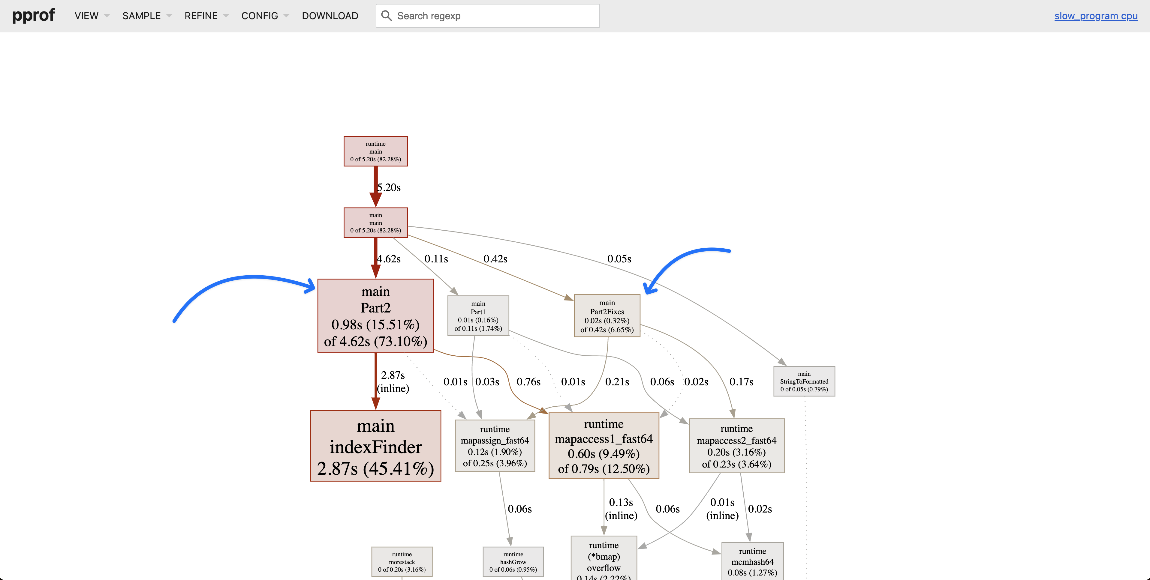
Graph View: This shows a directed graph of function calls. Nodes are functions, and their size represents the total CPU time spent in that function and any functions it called. The arrows show the call path, with thicker arrows representing hotter paths.

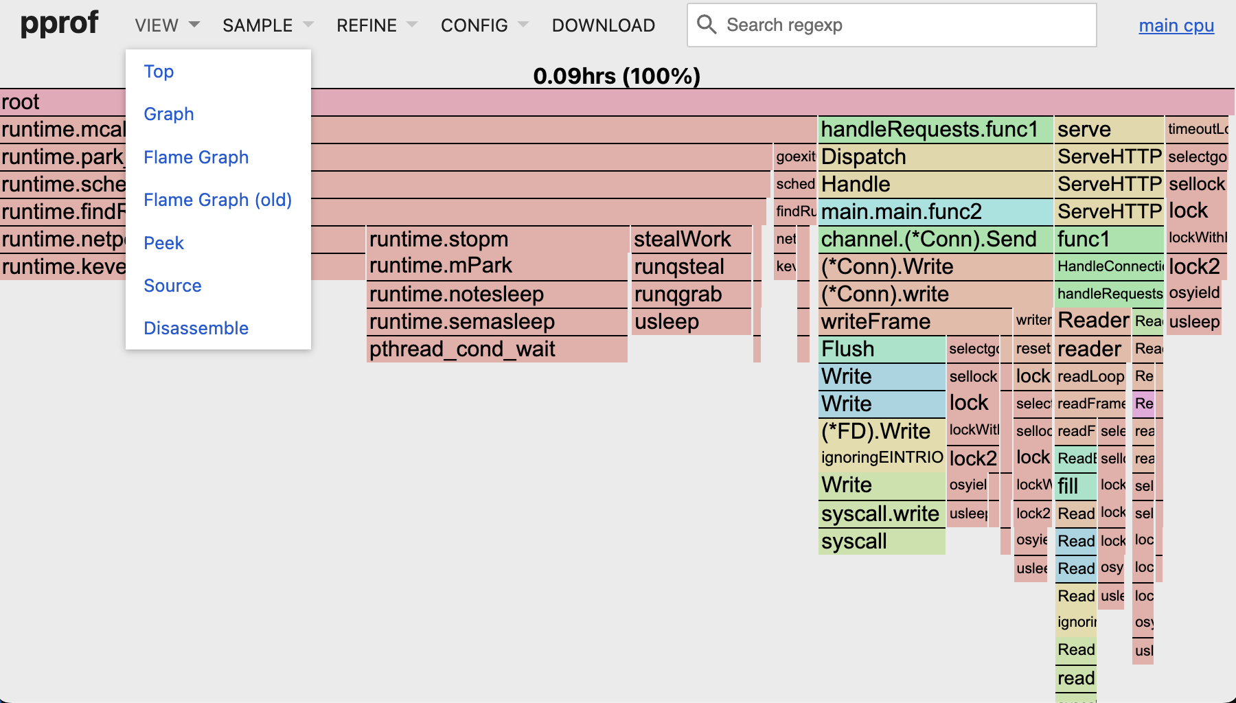
A pprof call graph. The wider nodes and thicker lines indicate "hot paths" where the program spends most of its CPU time. Your goal is to follow these heavy paths from `main` to the bottleneck.

Flame Graph View: This view excels at showing the call stack. The y-axis is the stack depth (what called what), and the x-axis represents the total samples (CPU time). Wider "plateaus" in the graph identify functions that are consuming significant CPU time.

Go pprof Flame Graph Visualization — The pprof flame graph view. Functions at the top of the stack (the top of a flame) that are wide are often the direct cause of CPU usage and are prime candidates for investigation.

A key principle in reading these graphs is to look for the largest contributors.

GopherCon 2019: Two Go Programs, Three Different Profiling Techniques - Dave Cheney

Dave Cheney provides an excellent demonstration of the core principle for reading pprof graphs in his GopherCon talk. This will help you orient yourself when looking at your own profile.

Watch from 22:21 to 24:36. Focus on his principle: 'when you're reading these graphs you follow the arrow... it tells you where most of the time is being spent.' This is the single most important rule for starting a CPU profile analysis.

2.2 Understanding the Full Picture

When you look at your profile, you'll see your application's functions (main.handleConnection, broker.(*Broker).handleProduceRequest, etc.), but you'll also see many runtime.* functions. A profile of a networked Go application is a story of your code interacting with the Go runtime (scheduler, garbage collector) and the operating system (syscalls for network and disk I/O).

Understanding these categories is crucial for correct interpretation.

Practical Example of Profiling Networked Go Applications with pprof

The article 'Practical Example of Profiling Networked Go Applications' provides a superb breakdown of a real CPU profile for a networked Go app. This will give you a vocabulary for interpreting what you see in your own broker's profile.

Please read the sections 'Where the Time Went' and 'Summary: CPU and Memory Profiling of the /gc Endpoint'. Pay close attention to how the analysis is broken down into four key areas: the HTTP stack, Garbage Collection, I/O and Syscalls, and Scheduler Activity. This will help you categorize the functions you see in your own profile.

2.3 Your Turn: Analyze the Broker's Profile

Now, apply these concepts to the profile you captured, which should be open in your browser at http://localhost:8081.

Start with the Graph view. Find the main.main or runtime.main box. Follow the thickest arrows. What is the main call path that seems to be consuming the most time? You will likely see a path through net/http (for the pprof server itself) and a much more interesting path for our broker, probably starting from main.handleConnection.
Switch to the Flame Graph view. Look for the widest bars. Are they related to your broker's logic, Go's runtime, or system calls? A wide bar at the very top of a call stack indicates a function that is directly consuming a lot of CPU. In a system like ours that performs I/O, it's common to see syscall.Write or syscall.Read appear as very wide bars.

Based on our broker's design, a likely hot path involves receiving a message, serializing it, and writing it to a file-based log. You might see a function like log.Append or os.(*File).Write consuming a significant percentage of CPU time.

2.4 From Function to Line: The Source View

Once you've identified a hot function, the final step is to pinpoint the exact line(s) of code responsible. The pprof UI makes this straightforward.

In either the Graph or Flame Graph view, click on one of the boxes representing a function from your own code (e.g., broker.handleProduceRequest or a method on your log storage). This will open a menu. Select Source.

The Source view displays the function's source code, annotated line-by-line with the amount of CPU time spent. The numbers in the columns are crucial:

flat: Time spent directly executing code on this line.
cum (cumulative): Time spent on this line plus time spent in any functions called from this line.

A high flat value on a single line is a classic hot spot.

Go (Golang) Profiling Tutorial

This short clip demonstrates how to go from a high-level view to the specific line of code causing a bottleneck using pprof's built-in tools.

Watch from 09:51 to 10:39. The presenter uses the list <function_name> command in the pprof terminal to view the annotated source. You can achieve the same result more easily by clicking on a function in the web UI and selecting 'Source'. The key takeaway is how this view immediately reveals the performance problem.

Action: Go back to your broker's profile in the browser. Find the function you identified as a hot spot and open its Source view.

Which line has the highest flat cost?
What is that line of code doing? Is it performing serialization (binary.Write)? Is it writing to disk (f.Write)?

Finding this line is the goal of our analysis. For example, if you find that a syscall.Write call inside your log's Append method is consuming most of the flat time, you've just proven that your performance is likely bound by how you perform disk I/O. This doesn't mean syscalls are "slow"; it means your application is making them very frequently. This insight would lead us to consider strategies like buffered writing, which we can explore later.

Conclusion

In this lesson, we took a deep, practical dive into CPU profiling. You've learned the complete workflow: generating load, capturing a live profile, and systematically analyzing it to find the code that's costing you performance.

Key Takeaways:

Profiling should always be done under a realistic load.
The go tool pprof web UI is a powerful interactive tool for analysis.
Start by using the Graph and Flame Graph views to identify hot functions by "following the time".
A profile includes your code, the Go runtime, and system calls; understanding each is key to correct interpretation.
Use the Source view to drill down from a hot function to the specific, high-cost lines of code.
The goal is to move from guessing to making data-driven decisions about where to focus your optimization efforts.

Next Up

We've focused on CPU time, but that's only half of the performance story. The other half is memory. In our next lesson, we will shift our focus and use pprof to capture and analyze a heap profile. This will help us understand our broker's memory allocation patterns, identify sources of garbage collection pressure, and check for potential memory leaks.

Recommended resources