Electric Field from Continuous Charge Distributions

1. The Strategy: From Discrete Sums to Continuous Integrals

In the previous lesson, we found the net electric field by performing a vector sum of the fields from individual point charges:

When we have a continuous object, we can't sum individual charges. The core idea is to imagine the object is made up of an infinite number of infinitesimally small charge elements, which we'll call $dq$. Each of these tiny elements acts like a point charge and creates a differential electric field, $d\vec{E}$, at the point of interest.

To find the total electric field, we simply "sum" up—or integrate—the contributions from all these infinitesimal elements over the entire object:

To make this practical, we need a way to define $dq$. We do this using the concept of charge density. For the objects in this lesson (lines and rings), we will use the linear charge density, $\lambda$, which is the charge per unit length (units: C/m). For a uniform distribution, $\lambda =Q/L$, where $Q$ is the total charge and $L$ is the total length.

An infinitesimal piece of the object with length $dl$ will then have a charge $dq=\lambda dl$. Our integral becomes:

The following reading introduces this powerful generalization from summation to integration.

The general strategy we will apply is:

1. Divide and Conquer: Break the charge distribution into infinitesimal elements $dq$.
2. Field of an Element: Write down the expression for the differential electric field $d\vec{E}$ from this element.
3. Exploit Symmetry: Analyze the geometry to see if any components of the electric field will cancel out. This is often the most important step for simplifying the problem.
4. Integrate: Set up and evaluate the integral for the non-canceling components of $d\vec{E}$ over the entire charge distribution.

2. Electric Field of a Finite Charged Rod

Let's apply this strategy to our first case: finding the electric field at a point P located a distance $z$ from the midpoint of a straight rod of length $L$ with a uniform linear charge density $\lambda$.

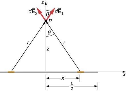
As the diagram shows, for every charge element $dq$ on the right side of the rod's center, there is a corresponding element on the left side at the same distance. The horizontal components of their electric fields ($d{E}_x$) are equal and opposite, so they cancel. The vertical components ($d{E}_z$) are equal and in the same direction, so they add up. Therefore, we only need to integrate the $z$-component of the field.

The detailed derivation involves setting up the integral and solving it, a process that requires careful application of calculus. The following reading walks you through this derivation step-by-step.

To see this entire process, including the calculus, explained in meticulous detail, the following video is an outstanding resource. It provides a full derivation from first principles and also mathematically proves that the perpendicular field components sum to zero, confirming our symmetry argument.

The final result for the field a distance $z$ from the center of a rod of length $L$ with total charge $Q=\lambda L$ is:

You are not expected to memorize this formula, but you should understand the method used to derive it.

3. Electric Field of a Charged Ring

Next, let's find the electric field at a point P on the axis of a uniformly charged ring of radius $R$ and total charge $Q$. The point P is a distance $x$ from the center of the ring.

The symmetry here is even more powerful than for the rod. As the diagram shows, for any charge element $dq$ on the ring, there is another one directly opposite it. The components of their electric fields perpendicular to the axis cancel each other out. Only the components along the axis (the $x$-axis in the diagram) contribute to the net field.

This simplifies the integration significantly. The distance $r=\sqrt{R^2+x^2}$ from any charge element $dq$ to the point P is constant. The angle $\theta$ is also constant for all elements. This means the factors $1/r^2$ and $\cos \theta$ can be taken outside the integral!

The following reading provides the concise derivation.

The final result for the field on the axis of a ring is:

Again, the derivation process is more important than memorizing the final formula.

4. Conceptual Checks: Limiting Cases

A powerful way to build physical intuition and check your results—a common technique in exams—is to test them in limiting cases.

• Far-Field Limit ($x\gg R$ or $z\gg L$): What should the field of the rod or the ring look like from very far away? From a great distance, any finite object should look like a point charge. Let's check our formula for the ring. If $x\gg R$, then $x^2+R^2\approx x^2$.

  $$E_x=k\frac{Qx}{(x^2{)}^{3/2}}=k\frac{Qx}{x^3}=k\frac{Q}{x^2}$$

  This is exactly the formula for the electric field of a point charge $Q$. The formula behaves as expected! You can perform a similar check for the finite rod formula.

• Center of the Ring ($x=0$): What is the field at the exact center of the ring? By symmetry, the field contributions from all the opposite pairs of charges must cancel perfectly. The net field should be zero. Let's check our formula: if we set $x=0$, the numerator becomes zero, so $E_x=0$. It works.

• Infinite Line Limit ($L\to \infty$): What if our finite rod becomes infinitely long? This is an important theoretical case. In the OpenStax text, just after the finite rod example, the derivation is extended to an infinite line.
  The result is $E=\frac{k\lambda }{z}\cdot 2$, or more commonly written as $E=\frac{1}{2\pi {ϵ}_0}\frac{\lambda }{z}$. Notice the field from an infinite line decreases as $1/z$, not $1/z^2$. This is a unique feature of its geometry.

Conclusion

In this lesson, we bridged the gap between discrete charges and continuous objects. By combining the superposition principle with calculus, you now have a universal method to calculate electric fields for any shape.

Here are the key takeaways:

• The electric field of a continuous charge distribution is found by integrating the differential field elements $d\vec{E}$ over the object: $\vec{E}=\int d\vec{E}$.
• The charge element $dq$ is defined using charge density, such as linear charge density $\lambda$, where $dq=\lambda dl$.
• Symmetry is your most powerful tool. Always analyze the geometry first to see which field components will cancel, as this drastically simplifies the integration.
• We derived the expressions for the electric field of a finite rod and a charged ring on its axis. We also saw how to verify these results using limiting cases.

In our next lesson, we will introduce a new, and in some ways more elegant, law for calculating electric fields: Gauss's Law. While our integration method today works for any shape, it can be mathematically complex. Gauss's Law provides a stunningly simple shortcut for calculating the field of distributions with high degrees of symmetry, such as the infinite line we just considered.