Hello! In our last lesson, we explored the mechanics of the discrete convolution, seeing how learnable kernels act as feature detectors that slide across an input to produce feature maps. While powerful, this process leaves us with two challenges: the resulting feature maps can be computationally large, and they are sensitive to the exact location of the features they detect.
In this lesson, we will introduce the solution to these challenges: the pooling layer. You will learn how simple, non-learnable operations like Max Pooling serve the dual purpose of reducing computational complexity and creating a degree of translation invariance. This makes the network's representations more robust and efficient, a cornerstone of modern CNN architectures.
What is Pooling? A Mechanism for Downsampling
At its core, a pooling layer is a method for downsampling a feature map, reducing its spatial dimensions (height and width) while aiming to retain the most important information. Unlike convolutional layers, pooling layers have no learnable parameters. They perform a fixed operation on small regions of the input.
The two most common types of pooling are:
- Max Pooling: For each region (or "pooling window"), the operation outputs the maximum value from that region.
- Average Pooling: For each region, the operation outputs the average of all values in that region.
The pooling operation slides a window across the input feature map, just like a convolution. However, instead of a weighted sum, it applies the max or average function. The most common configuration is a 2x2 pooling window with a stride of 2. This has the effect of reducing the height and width of the feature map by half, thus quartering the total number of activations.
The image below shows a direct comparison of Max Pooling and Average Pooling on a 4x4 feature map.
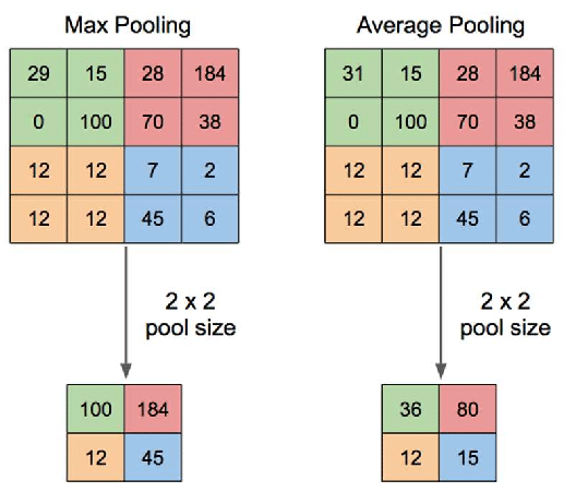
A comparison of a 2x2 Max Pooling and a 2x2 Average Pooling operation. Max Pooling selects the highest value from each 2x2 block (e.g., max(29, 15, 0, 100) = 100), while Average Pooling calculates the mean (e.g., avg(31, 15, 0, 100) ≈ 36).
To begin, let's watch a short video that introduces the concept of pooling and compares the Max and Average pooling operations.
What are Pooling Layers in Deep Neural Networks?
This video, "What are Pooling Layers in Deep Neural Networks?", clearly outlines the primary motivations for using pooling and explains the mechanics of the two main types.
Please watch from the beginning until the end of the comparison. Pay attention to the three main reasons given for using pooling, and the described benefits and downsides of both Max Pooling and Average Pooling.
As you saw, Max Pooling tends to be preferred in most modern architectures. Its key advantage is that it captures the most salient signal—the strongest activation—from a local region. This implies that the layer is most interested in whether a feature was detected, rather than the average strength of all features in that region.
The First Benefit: Reducing Computational Load
The most immediate benefit of pooling is dimensionality reduction. By decreasing the spatial size of the feature maps, we dramatically reduce the computational burden for the rest of the network.
Consider a typical CNN where we stack multiple convolutional layers. Without pooling, the feature maps would remain large, and each subsequent convolutional layer would have to perform a massive number of calculations. By inserting a pooling layer after a convolutional layer, we shrink the feature map. This means the next convolutional layer will:
- Have a smaller input to process.
- Require fewer parameters if it's a fully-connected layer down the line.
- Have a larger effective receptive field on the original image for the same kernel size, a concept we'll explore in a later lesson.
Let's return to the video to see a visualization of how this plays out in a real network architecture like Google's InceptionNet.
What are Pooling Layers in Deep Neural Networks?
The video provides an excellent illustration of how pooling layers are used to manage complexity in deep networks.
Watch the segment on dimensionality reduction, from this timestamp. Notice how the spatial dimensions (height and width) decrease while the number of channels (filters) often increases in deeper layers. Pooling is what makes this architectural pattern computationally feasible.
The Second Benefit: Creating Translation Invariance
The second, more subtle benefit of pooling is that it introduces translation invariance. This is a critical property for tasks like image classification, where an object's identity doesn't change if it's shifted slightly.
To understand this, we must first distinguish it from the translation equivariance of convolutional layers. As we saw, if you shift the input to a convolutional layer, the feature map shifts by the same amount. The pattern of activations moves with the input.
Invariance is different: it means that if you shift the input slightly, the output does not change. Max pooling provides a localized version of this property. Because it only reports the maximum value within a pooling window, it doesn't care about the exact position of the activation, only its presence. If a feature detector activates and then shifts slightly but remains the strongest signal within the same pooling window, the output of the max pooling layer will be identical.
The following image and the accompanying article provide a brilliant and intuitive explanation of this effect.
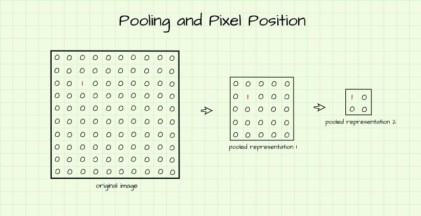
An illustration of how two pooling operations reduce the spatial dimensions of an image. A single active pixel in the original image is mapped to a different location in the final 2x2 representation depending on its initial position.
Now, let's read the article that this image comes from. It walks through a simple "from scratch" example using a single active pixel to demonstrate how max pooling makes the network's representation robust to the feature's position.
Translation Invariance & Equivariance in Convolutional Neural Networks
This blog post from Paperspace provides a clear, code-supported explanation of how pooling layers create translation invariance.
Start by reading the introduction to refresh the distinction between translation invariance and equivariance. Then, skip down to the section titled "Image 1". Follow the excellent example that tracks a single active pixel. Read through the text and visualizations for "Image 1" and "Image 2". Finally, read the crucial "Comparing Images" section. This is where the concept clicks: it shows how, after several pooling steps, the representations of two differently placed features become much closer, achieving invariance. Read from this paragraph.
As the article demonstrates, while a single pooling operation provides only very local invariance, stacking multiple conv-pool blocks causes this effect to aggregate. Over the depth of the network, the representation becomes increasingly insensitive to the precise location of features, focusing instead on their presence and relative spatial configuration.
This distinction is key:
- Convolutional layers are equivariant to translation, preserving location information.
- Pooling layers introduce invariance to translation, discarding precise location information in favor of robustness.
The following short clip offers another concise way to think about this distinction.
Equivariant Neural Networks Part 13 - Introduction
This video provides a very quick and clear definition of invariance and connects it directly to pooling.
Watch the short segment from this timestamp. The idea of pooling as a "set function" (like max or mean) that doesn't care which specific element produced the result is a powerful mental model for invariance.
Pooling Mechanics in Practice
Now that we understand the "why," let's solidify the "how." The "Dive into Deep Learning" textbook provides a clear, practical summary and a from-scratch implementation.
7.5. Pooling — Dive into Deep Learning 1.0.3 documentation
This chapter of the online textbook "Dive into Deep Learning" covers the essential mechanics of pooling layers.
First, read the introductory section to see how pooling fits into the broader context of CNNs: 7.5. Pooling. Next, review the section on "Maximum Pooling and Average Pooling", which includes a helpful diagram and the explicit calculation for a max-pooling operation. Read from this section. Then, examine the from-scratch Python implementation in the code block under the text. You don't need to run it, but studying the pool2d function will solidify your understanding of the sliding window mechanism: the pool2d function. Finally, read the Summary section, which concisely recaps the key properties of pooling layers: 7.5.4. Summary.
Conclusion
In this lesson, we've added a crucial tool to our CNN toolkit: the pooling layer. While simple, its impact on a network's architecture and performance is profound.
- Key Takeaways:
- Pooling layers perform a downsampling operation (e.g., max or average) on feature maps using a sliding window with no learnable parameters.
- Their primary function is to reduce the spatial dimensions of feature maps, which decreases the computational load and number of parameters in subsequent layers.
- Max Pooling, the most common type, introduces a degree of local translation invariance. It makes the network more robust to small shifts in feature locations by capturing the presence of a feature rather than its exact position.
- A common configuration of a
2x2window with a stride of2quarters the size of the input feature map.
We have now examined the three core components of a standard CNN block: the convolutional layer for feature detection, the non-linear activation function for learning complex patterns, and the pooling layer for efficiency and invariance.
In our next lesson, we will put all these pieces together. We will trace the complete flow of data through a simple, complete CNN architecture to see how an input image is transformed into a set of powerful, abstract feature maps.