Data Flow in CNNs: From Input to Feature Maps

Hello! Welcome back to our course.

In our previous lessons, we individually examined the essential building blocks of Convolutional Neural Networks: the convolutional layer for detecting features, the ReLU activation function for introducing non-linearity, and the pooling layer for creating efficiency and local invariance. Now it's time to assemble these components and see how they work together in a complete system.

This lesson addresses the learning outcome: Trace the flow of data through a simple Convolutional Neural Network (CNN) to produce a set of feature maps. We will follow an input image on its journey through the network, observing how it is transformed at each stage. By the end, you'll have a clear, end-to-end mental model of how a CNN processes visual information, moving from raw pixels to a rich, hierarchical set of features.

The Anatomy of a Modern CNN

A typical CNN for image processing consists of two main parts: a feature extraction frontend and a classification backend. The feature extraction part is a sequence of blocks, where each block usually contains a convolutional layer, a non-linear activation (like ReLU), and a pooling layer. This is the part we'll focus on. The classification backend usually consists of one or more fully-connected layers that take the final feature maps, flatten them into a vector, and make a prediction.

Let's look at the architecture of VGG-16, a classic deep CNN.

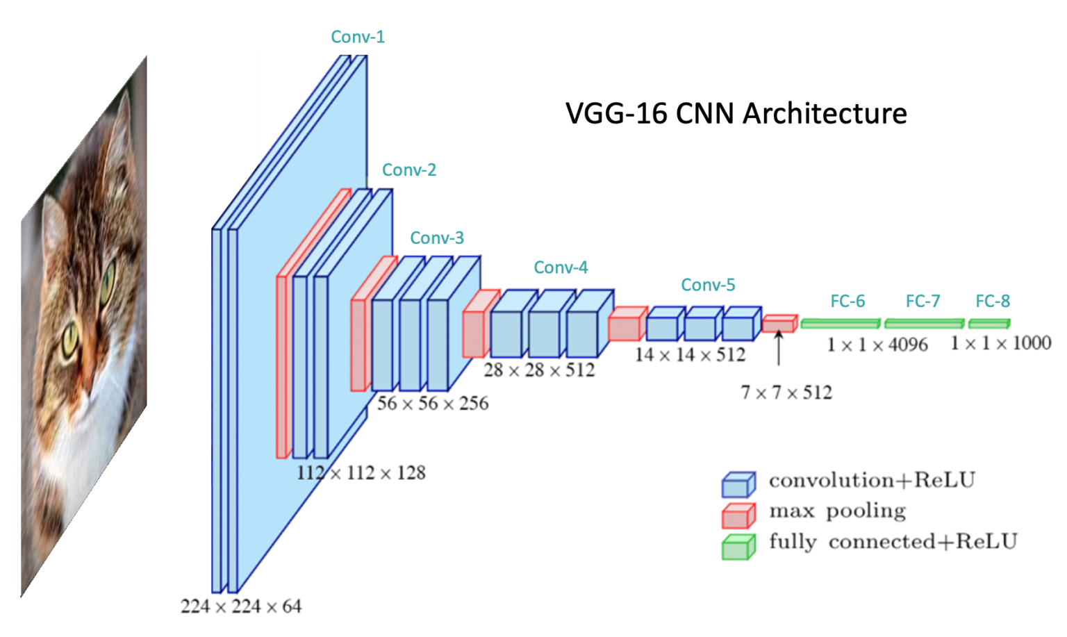
The architecture of the VGG-16 network. An input image is processed by a series of convolutional, ReLU, and max pooling layers. Notice the pattern: as the data flows from left to right, the spatial dimensions (height and width) of the feature maps decrease, while the depth (number of channels) increases.

While VGG-16 is deeper than the "simple" CNN we'll dissect today, it perfectly illustrates the fundamental principle. It's composed of repeating Convolution + ReLU blocks followed by Max Pooling layers. This structure systematically transforms a spatial representation (the image) into a feature-based representation.

A Visual Trace Through a Simple CNN

The most intuitive way to understand the data flow is to watch it happen. The following video provides an excellent animated visualization of an MNIST handwritten digit being processed by a simple CNN. This will help build a strong visual foundation for the entire process.

Visualizing Convolutional Neural Networks | Layer by Layer

This video, "Visualizing Convolutional Neural Networks | Layer by Layer," provides a clear, step-by-step animation of the data transformations inside a CNN.

Please watch the entire video from start to finish. As you watch, pay close attention to the following stages: First Convolution (Conv1): Observe how the two separate filters process the single input image to create two distinct feature maps (channels). First Pooling (Pool1): See how max pooling downsamples each feature map independently, reducing their spatial dimensions. Second Convolution (Conv2): This is a crucial step. Notice how each of the four new filters has a depth of 2, allowing them to process information from both channels of the preceding layer to produce a new output channel. Flattening & Prediction (Flatten/FC): Watch how the final stack of 2D feature maps is unrolled into a 1D vector to be fed into the final classification layer.

This visualization makes the abstract process tangible. We start with a recognizable image of a '7'. After the first convolution, we can still discern some shapes. By the end of the second convolution, the representation is no longer visually interpretable to us as a digit. Instead, it's a set of abstract feature activations that the network uses for classification.

A Code-Based Trace: The Forward Pass

Given your background, seeing the data flow defined in code can provide an even clearer and more precise understanding. The forward method of a neural network module in frameworks like PyTorch or TensorFlow defines this exact sequence of operations.

Let's examine a practical implementation from the article "The Math Behind Convolutional Neural Networks." This article builds a simple CNN in PyTorch for the MNIST dataset, very similar to the one in the video.

The Math Behind Convolutional Neural Networks

This article provides a thorough breakdown of CNNs, including a complete code example. We will focus on the forward method, which programmatically defines the data flow.

Please scroll down to section "3.3: Designing the CNN Model". First, familiarize yourself with the network's structure by reading the code block that defines the MyCNN class, from the class definition. Now, focus on the forward method. Read the code and the accompanying step-by-step explanation, starting from the final paragraph. This section perfectly maps the sequence of operations you just saw in the video to their corresponding lines of code.

The forward method is the heart of the network's execution. Each line directly corresponds to a transformation of the data tensor x:

x = F.relu(self.conv1(x)): Pass through the first convolutional layer, then apply ReLU.
x = F.max_pool2d(x, 2, 2): Apply max pooling.
x = F.relu(self.conv2(x)): Pass through the second convolutional layer, then apply ReLU.
x = F.max_pool2d(x, 2, 2): Apply max pooling again.
x = x.view(x.size(0), -1): Flatten the 3D feature maps into a 1D vector.
x = F.relu(self.fc1(x)) and x = self.fc2(x): Pass through the fully connected layers for classification.

This sequence is the fundamental pattern of a feature-extracting CNN.

A Mathematical Trace: Calculating Feature Map Dimensions

To complete our understanding, let's trace the flow with a pen-and-paper calculation. We'll use the classic LeNet-5 architecture as an example and calculate the exact dimensions of the feature maps at each step. The formula for the output size of a convolutional or pooling layer is:

Output Size = \frac{( Input Size - Kernel Size + 2 \times Padding )}{Stride} + 1

The following article provides a clear, step-by-step walkthrough of this calculation.

How CNNs Process an Image: A Deep Dive into Feature ...

This article offers a concise breakdown of feature map calculations using the LeNet-5 architecture as a case study.

Please read the section titled "Mathematical Breakdown of Feature Map Calculation". Focus on the paragraph that traces the dimensions layer by layer, starting from the breakdown of LeNet-5.

Let's summarize the flow described in the article:

Input: A 32x32x1 grayscale image.
CONV1: Applies 6 filters of size 5x5 with a stride of 1.
- Output width/height: ((32 - 5) / 1) + 1 = 28.
- Output volume: 28x28x6.
POOL1: Applies 2x2 max pooling with a stride of 2.
- Output width/height: ((28 - 2) / 2) + 1 = 14.
- Output volume: 14x14x6.
CONV2: Applies 16 filters of size 5x5 with a stride of 1.
- Output width/height: ((14 - 5) / 1) + 1 = 10.
- Output volume: 10x10x16.
POOL2: Applies 2x2 max pooling with a stride of 2.
- Output width/height: ((10 - 2) / 2) + 1 = 5.
- Final feature maps: 5x5x16.

At this point, the network has successfully transformed the 32x32 pixel grid into a 5x5x16 volume of feature activations. This compact, dense representation is what the subsequent fully connected layers will use to make a final decision.

What Do These Feature Maps Represent?

We've traced how feature maps are created. But what are they? They are hierarchical representations of the input image. Early layers learn to detect simple patterns, and deeper layers compose these simple patterns into more complex ones.

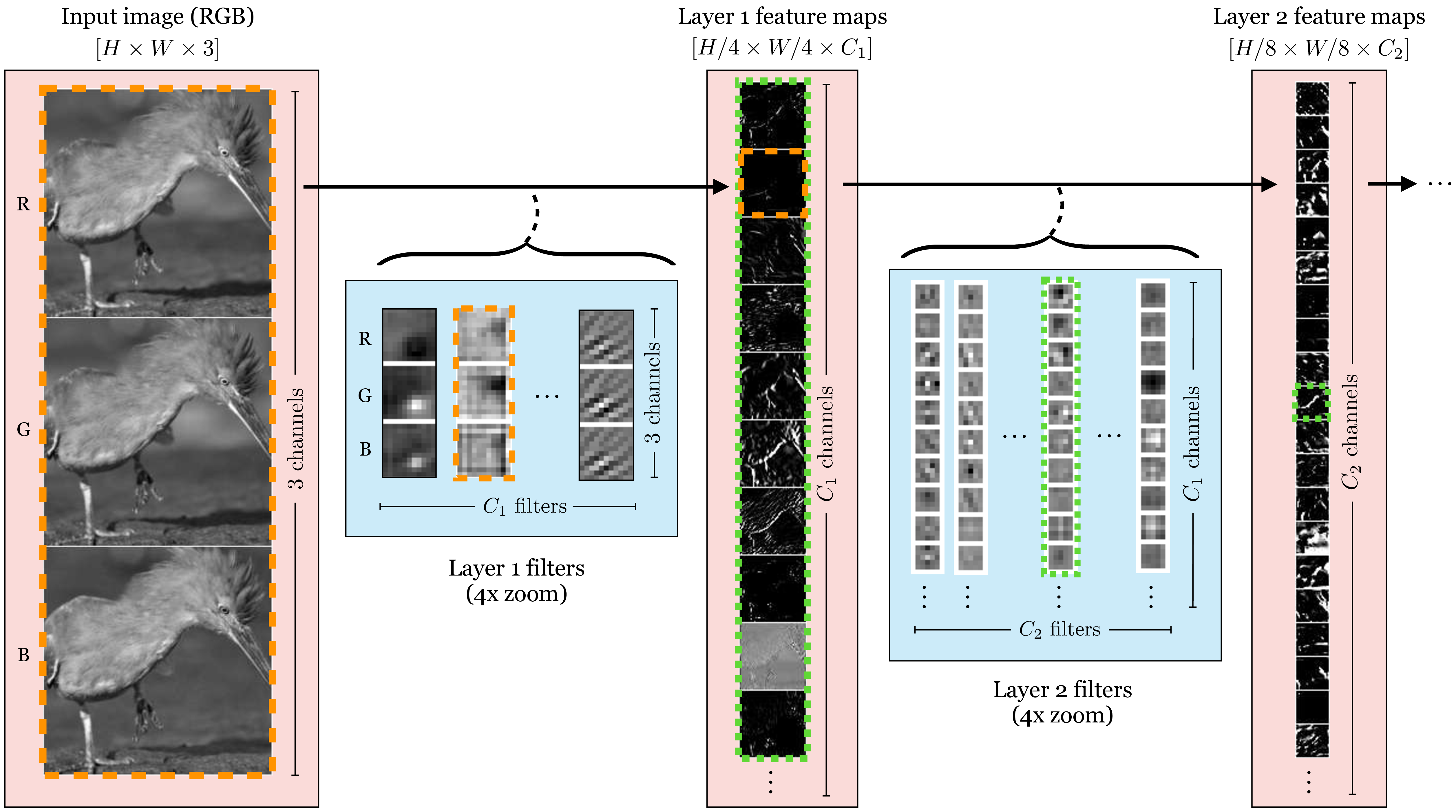
An illustration of hierarchical feature extraction. Layer 1 filters learn to detect simple edges and color gradients. Layer 2 filters combine the activations from Layer 1 to detect more complex textures and patterns, like the patterns on the bird's feathers.

This hierarchical learning is the "magic" of deep learning. The network learns the features automatically from data. In the first layer, filters might learn to be detectors for horizontal, vertical, and diagonal edges. In the next layer, filters might learn to combine these edge detections to find corners, curves, or simple textures. In a network trained to recognize faces, even deeper layers might learn to activate for eyes, noses, and mouths, just as this MIT lecture clip illustrates.

MIT 6.S191: Convolutional Neural Networks

This clip from an MIT lecture on CNNs beautifully visualizes the learned filters at different depths of a face detection network.

Watch the segment from this timestamp. You'll see a clear progression from simple edge detectors in the early layers to complex feature detectors (eyes, noses) in the mid-layers, and finally to representations of entire faces in the late layers.

Conclusion

In this lesson, we synthesized our knowledge of individual CNN components to understand the full data flow.

Key Takeaways:
- A CNN processes an input image through a sequence of blocks, typically containing convolution, activation (ReLU), and pooling layers.
- Data flows through the network as a 3D volume (height x width x channels).
- Convolutional layers apply filters to create new feature maps. The number of filters determines the depth (number of channels) of the output volume.
- Pooling layers downsample the feature maps, reducing their spatial dimensions (height and width) while keeping the depth the same.
- This process creates a hierarchy of features: early layers detect simple patterns like edges, while deeper layers combine these to detect more complex, abstract concepts.

We have now seen how a CNN transforms an image into a set of feature maps. In our next and final lesson for this module, we will explore the concept of the receptive field, which explains what a single neuron at any given layer is "seeing" with respect to the original input image. This will complete our fundamental understanding of spatial feature learning in CNNs.