Understanding Discrete Convolution and Feature Map Transformation

The Convolution as a Sliding Dot Product

At its heart, a 2D discrete convolution is a straightforward operation. It involves a small matrix called a kernel (or filter) and a larger matrix representing the input (e.g., a grayscale image or a feature map from a previous layer). The operation systematically combines these two to produce an output feature map.

The process works as follows:

1. The kernel is placed over a region of the input map, starting at the top-left corner.
2. An element-wise multiplication is performed between the values in the kernel and the corresponding values in the patch of the input it covers.
3. All the results of these multiplications are summed up to produce a single number.
4. This single number becomes the first value in the output feature map.
5. The kernel then slides over to the next position (e.g., one pixel to the right), and the process is repeated to compute the next value in the output map.

This "slide, multiply, sum" procedure continues until the kernel has covered the entire input.

The image below provides a static illustration of this calculation for a single output value. The 3x3 kernel is placed over a 3x3 patch of the source layer. The corresponding elements are multiplied and then summed to produce the value '5' in the destination layer.

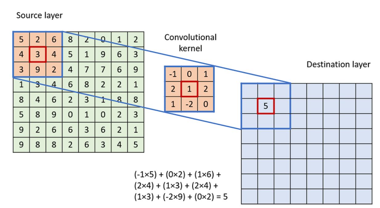
This diagram shows a 3x3 convolutional kernel processing a patch of a larger source layer. The value '5' in the destination layer is calculated by performing an element-wise product of the kernel and the underlying source patch, followed by a summation of the results.

To see this process in motion, the 3Blue1Brown video offers an exceptionally clear and intuitive explanation, building from simple 1D examples to 2D image applications.

The Effect of Convolution: Feature Detection

What is the purpose of this operation? The convolution acts as a feature detector. The values within the kernel determine what kind of pattern or feature it will "activate" on. When the pattern in the input patch closely matches the pattern in the kernel, the dot product will result in a large value (positive or negative). If the patterns don't match, the result will be close to zero.

The output feature map, therefore, is a spatial map of where the kernel's target feature was detected in the input.

A classic example is an edge detector. Consider a kernel designed to find vertical edges:

When this kernel is slid over a region of an image that is uniform (all the same color), the sum of products will be zero. However, if it slides over a sharp vertical edge (e.g., light pixels on the left, dark pixels on the right), the positive kernel values will multiply with the high pixel values and the negative kernel values with low pixel values, resulting in a large positive output.

The following video demonstrates this effect visually, showing how different hand-crafted kernels can detect vertical and horizontal edges or create blur effects.

In traditional computer vision, engineers would manually design these kernels. The breakthrough of Convolutional Neural Networks is that the values of the kernels are not pre-programmed; they are learnable parameters. Through backpropagation, the network learns the optimal kernel values to detect features that are most useful for solving a specific task (e.g., classifying an object, segmenting a region).

The Arithmetic of Convolutions: Controlling Output Size

The dimensions of the output feature map are a direct function of the input size and three key hyperparameters of the convolutional layer: padding, stride, and kernel size. Understanding this relationship is crucial for designing network architectures.

Let's define the terms:

• Input size (i): The height/width of the input feature map.
• Kernel size (k): The height/width of the kernel.
• Stride (s): The number of pixels the kernel slides at each step. A stride of 1 moves one pixel at a time, while a stride of 2 skips a pixel, effectively downsampling the output.
• Padding (p): The number of pixels (usually with value 0) added around the border of the input feature map.

The output size (o) can be calculated with the following formula:
$o=\lfloor \frac{i+2p-k}{s}\rfloor +1$

Padding is particularly important for two reasons:

1. It preserves spatial dimensions. Without padding, each convolutional layer would shrink the feature map. By adding the right amount of padding, we can ensure the output has the same height and width as the input. This is often called "same" padding. A common choice is p = (k-1)/2 for a stride of 1.
2. It allows features at the borders to be fully processed. Without padding, the pixels at the very edge of the image are only ever covered by the kernel once, while pixels in the center are covered many times. Padding ensures the kernel can be centered on every pixel of the original input.

The following paper provides a definitive guide to the arithmetic of convolutions.

Convolutions on Multi-Channel Inputs

So far, we've considered a single-channel (grayscale) input. Real-world images are typically RGB, having 3 channels. Similarly, hidden layers in a CNN can have many more channels (e.g., 64, 128, 256).

When applying a convolution to a multi-channel input, the kernel must have the same number of channels as the input. For instance, to convolve a 256 x 256 x 3 RGB image with a 5x5 kernel, the kernel's actual dimensions must be 5 x 5 x 3.

The convolution operation remains similar, but it is now a 3D dot product:

1. The 5 x 5 x 3 kernel is placed over a 5 x 5 x 3 patch of the input image.
2. An element-wise multiplication is performed across all 5 * 5 * 3 = 75 corresponding values.
3. All 75 products are summed up to produce a single value in the output feature map.

Crucially, a k x k x C_in kernel produces a single-channel (H_out x W_out x 1) output feature map. To generate an output with multiple channels (e.g., C_out = 64), you must apply C_out independent kernels to the same input. Each kernel learns to detect a different feature.

A Note on Convolution vs. Cross-Correlation

There's a subtle but important technical distinction to be aware of. The formal mathematical definition of convolution, as used in signal processing and probability theory, involves flipping the kernel by 180 degrees before the sliding dot product. This is the "flip and slide" operation you saw in the 3Blue1Brown video.

However, most deep learning libraries (including TensorFlow and PyTorch) implement what is technically cross-correlation, which is the same operation but without flipping the kernel.

Why is this acceptable? Because the kernel's weights are learned. If the optimal computation requires the flipped version of a kernel, the network is free to learn those flipped weights during training. From a functional perspective of a learnable feature extractor, the initial state (flipped or not) is irrelevant. It simply changes the interpretation of the learned weights, but not the expressive power of the layer.

Conclusion

In this lesson, we have dissected the fundamental operation of a discrete convolution.

• Key Takeaways:
  • A convolution is a linear operation that computes a sliding dot product between an input feature map and a smaller matrix called a kernel.
  • The kernel acts as a feature detector; its values determine the pattern it responds to. In a CNN, these kernels are learned automatically.
  • The output feature map is a spatial representation of where the kernel's feature was detected in the input.
  • Hyperparameters like stride and padding are crucial tools for controlling the spatial dimensions of the output feature maps.
  • For multi-channel inputs, the kernel must also be multi-channel, and the operation collapses the channel dimension, requiring multiple independent kernels to produce a multi-channel output.

We have now examined the two primary components of a convolutional layer: the convolution itself and the activation function. In our next lesson, we will introduce pooling layers, another essential building block in CNNs. We will explore how operations like Max Pooling reduce the computational load and help the network build representations that are robust to small shifts and distortions in the input image.