Welcome back! In our previous lesson, we established why convolutional layers, with their principles of local connectivity and parameter sharing, are vastly more efficient and effective for image data than fully-connected layers. We concluded by noting that these operations—convolutions and matrix multiplications—are fundamentally linear. However, the world, and especially the patterns within images, is profoundly non-linear.
This lesson addresses that crucial gap. We will explore the role of non-linear activation functions, such as the widely-used Rectified Linear Unit (ReLU). You will learn why a neural network without non-linearity is surprisingly limited and how adding these simple functions unlocks the ability to model the complex relationships essential for tasks like image analysis and generation. This foundational concept is key to understanding not just simple CNNs, but also the advanced generative models we'll be studying later.
The Linearity Trap
Let's begin with a thought experiment. What if we build a "deep" network by simply stacking multiple linear layers one after another? It seems intuitive that more layers should add more representational power. However, this intuition is misleading.
A short, clear video from the DeepLearning.AI course by Andrew Ng explains why. The core takeaway is that a composition of linear functions is, itself, just another linear function.
Why Non-linear Activation Functions (C1W3L07)
Please watch this excerpt from the video "Why Non-linear Activation Functions". It provides a concise mathematical argument for why non-linearity is essential.
Watch from the beginning to the main explanation. Pay close attention to the derivation around this mark, which shows how a two-layer linear network collapses into a single linear transformation.
As the video demonstrates, stacking linear layers is computationally wasteful; the entire multi-layer network can be mathematically reduced to a single layer. This means that no matter how many layers deep your network is, if it only contains linear operations, it can only learn linear relationships. It is no more powerful than a simple linear or logistic regression model.
To make this concrete, let's consider a classic problem that linear models cannot solve: the XOR function.
A Fresh Look at Nonlinearity in Deep Learning
This article from Towards Data Science provides an excellent walkthrough of why linear models fail at the XOR problem and how a simple non-linearity solves it.
Please read the introduction and the section "The Traditional Explanation". Note how the linear regression model fails completely, while a tiny network with a single ReLU activation function learns the non-linear XOR relationship perfectly.
Unleashing Complexity with Activation Functions
The solution to this limitation is to introduce a non-linear activation function after each linear layer (e.g., after each convolutional or fully-connected layer). This function takes the result of the linear operation (a weighted sum of inputs) and transforms it non-linearly.
This simple addition has a profound effect. It breaks the chain of linearity, allowing the network to build progressively more complex, non-linear representations of the data with each subsequent layer.
The animated image below provides a striking visual comparison. It shows two simple networks attempting to classify a dataset where the two classes are not separable by a single straight line.

This animation contrasts the decision boundary of a neural network with a non-linear activation function (left) against one without (right). The network without an activation function can only learn a linear boundary, failing to separate the 'two moons' data, while the non-linear network learns a curved boundary that successfully classifies the data.
The network without the activation function is powerless; its decision boundary remains a straight line. The network with the activation function, however, can bend and shape its decision boundary to fit the complex structure of the data.
How ReLU Creates Complexity from Simplicity
One of the most popular and effective activation functions today is the Rectified Linear Unit (ReLU). Its definition is surprisingly simple:
If the input is positive, it passes through unchanged. If it's negative, it becomes zero. How can this simple "switch" enable the learning of complex patterns?
The key insight is that a neural network combines many of these simple ReLU units. Each unit can be thought of as creating a "bent line." By adding, stretching, and flipping these bent lines, the network can approximate any continuous function. The StatQuest video below gives a fantastic visual intuition for this process.
Neural Networks Pt. 3: ReLU In Action!!!
This video, "ReLU In Action!!!", provides a step-by-step visualization of how a network combines simple ReLU outputs to fit complex data.
Watch the segment from this timestamp. Focus on how the simple "bent blue line" and "straight orange line" from individual neurons are added together to create the "green wedge" shape, which fits the data much better than a single line could. The final summary at the end is a key takeaway.
This ability to approximate complex functions by combining simple non-linearities is a cornerstone of deep learning, formalized by the Universal Approximation Theorem. This theorem states that a neural network with a single hidden layer containing a finite number of neurons with non-linear activation functions can approximate any continuous function to any desired degree of accuracy.
The image below illustrates this principle perfectly. By increasing the number of ReLU units, the network's approximation of a complex sine wave becomes progressively more accurate.
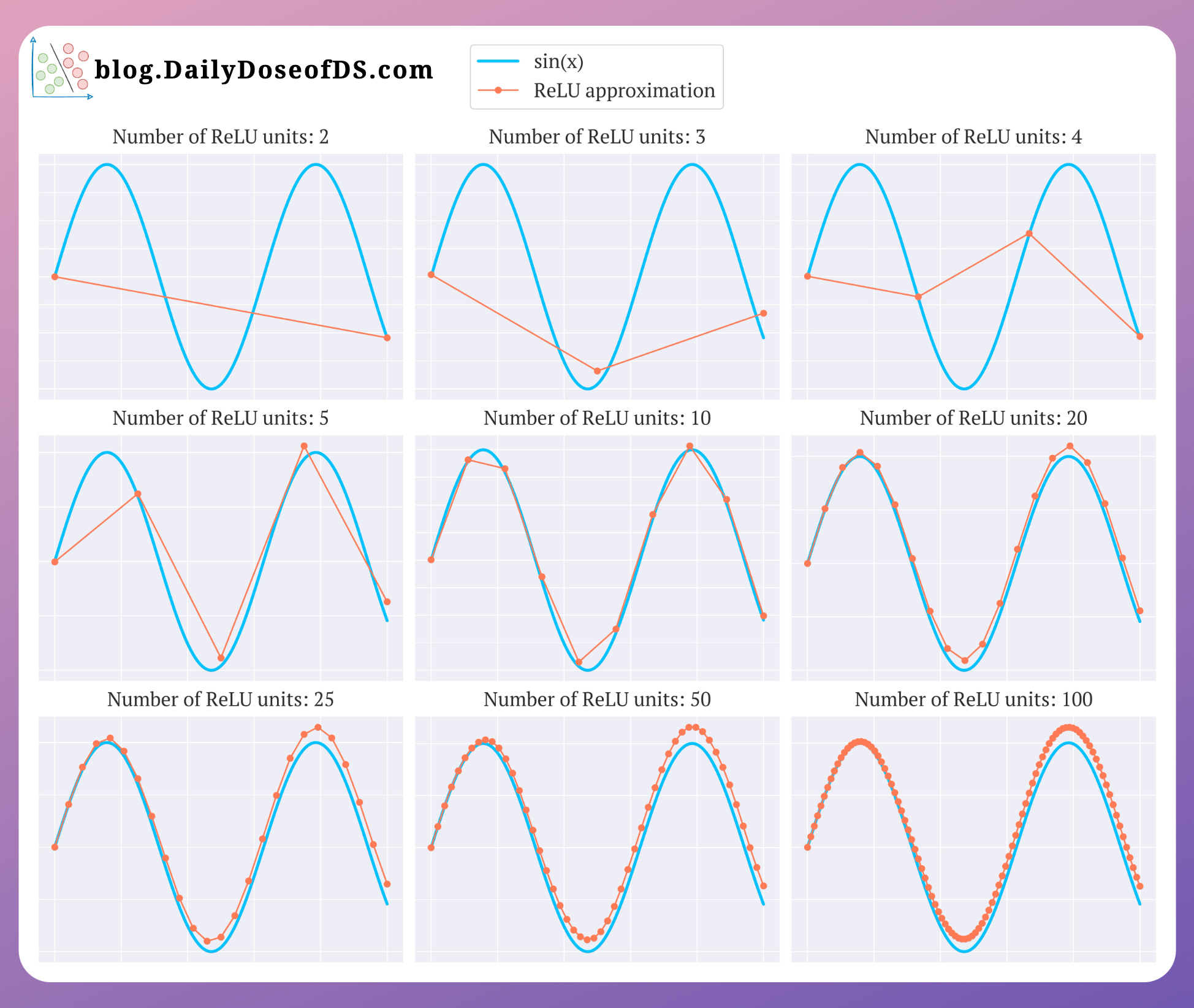
As the number of ReLU units increases from 2 to 100, the piecewise linear approximation (orange) becomes a progressively better fit for the non-linear sine wave (blue). This demonstrates the power of combining many simple non-linear functions.
A Deeper Perspective: Transforming Data for Linear Separability
Here is another, more profound way to think about the role of non-linear layers, which will resonate with your machine learning background. Instead of thinking about the network as just fitting a function to the data, think of the hidden layers as learning a transformation of the data.
The goal of these transformations is to take the raw input data, which might be a tangled, non-linearly separable mess, and warp it into a new high-dimensional space where the classes are linearly separable. The final layer of the network can then be a simple linear classifier that draws a hyperplane to separate the transformed data points.
A Fresh Look at Nonlinearity in Deep Learning
Let's return to the Towards Data Science article to explore this deeper perspective.
Please read the section titled "Digging Deeper: Inductive Bias". The key idea is that the final linear layer creates an "inductive bias" that forces the preceding non-linear layers to learn a representation that is linearly separable.
This viewpoint is incredibly powerful. It explains how deep networks work: they are a sequence of feature extractors that progressively untangle the data until a simple linear decision is possible.
A Quick Tour of Activation Functions and Their Issues
While ReLU is the modern default, it's worth knowing about other activation functions and their trade-offs.
-
Sigmoid and Tanh: Before ReLU, functions like the logistic (sigmoid) and hyperbolic tangent (tanh) were common. However, they suffer from the vanishing gradient problem. As the input to these functions becomes very large or very small, the function "saturates" and its derivative approaches zero. During backpropagation, these near-zero gradients are multiplied through the layers, causing the error signal to "vanish" and effectively halting learning in the early layers of a deep network.
-
The "Dying ReLU" Problem: ReLU helps mitigate the vanishing gradient problem for positive inputs (where its gradient is a constant 1). However, it has its own issue. If a neuron's input is consistently negative, it will always output zero, and its gradient will also be zero. This neuron is effectively "dead"—it can no longer participate in learning because no gradient flows through it.
The Baeldung article on activation functions provides a good overview of these issues.
Nonlinear Activation Functions in a Backpropagation Neural Network | Baeldung on Computer Science
This article gives a technical summary of the problems associated with sigmoid functions and the ReLU family.
Focus on the sections 5.11. Problems of the Sigmoid Activation Functions and the discussion of the Dying ReLU problem in section 6.2. This will clarify the motivations for moving from sigmoids to ReLUs, and for developing variants of ReLU.
To address the dying ReLU problem, variants like Leaky ReLU were introduced. Leaky ReLU gives a small, non-zero slope for negative inputs, ensuring that a gradient can always flow backward, even if a neuron's input is negative.
Key Takeaways
- A stack of linear layers is equivalent to a single linear layer. Neural networks require non-linear activation functions to learn complex, non-linear patterns.
- Activation functions like ReLU act as simple switches that, when combined across many neurons and layers, allow a network to approximate any continuous function.
- A deeper perspective is that non-linear layers work to transform input data into a new representation where the classes are linearly separable.
- Different activation functions have different properties and trade-offs. ReLU is computationally efficient and mitigates the vanishing gradient problem but can suffer from the "dying ReLU" problem, which variants like Leaky ReLU address.
In the last two lessons, we've covered the two essential components of a modern convolutional layer: the linear convolution operation and the non-linear activation. In our next lesson, we will dive deeper into the mechanics of the convolution itself, examining the mathematical operation of a discrete convolution and how it acts on an input feature map to produce a new one.