Hello. This module turns from how school calendars are arranged to what evidence about learning can—and cannot—show. A calendar can redistribute instructional days without adding any, so a smaller summer setback would not, by itself, establish a larger gain over the whole year.
In this lesson, you will read seasonal achievement graphs in three distinct ways: whether scores fall, whether scores rise more slowly, and whether the distance between student groups grows. Keeping those claims separate is essential when evaluating arguments for a different school calendar.
A summer slowdown is not always a summer decline
Imagine a test scale on which a group’s average score is 40 in fall and 60 the following spring. If its next fall average is 60, scores flattened over summer: there was no measured gain, but no measured decline. If the next fall average is 55, scores declined. Both patterns differ from the faster growth observed during the preceding school months.
Start with the distinction between these patterns in the Brookings article. The accompanying chart reports changes over summer, rather than students’ total scores.
Is summer learning loss real, and does it widen test score gaps by family income? | Brookings
Read this Brookings article for its distinction between summer scores that flatten and scores that drop.
Under “Multiple assessments indicate that test scores flatten or drop during the summer,” read the paragraph beginning “Across these studies”. Then inspect Figure 1 immediately below it. Stop before the paragraph beginning “These studies consistently show.” Focus on what the bars measure and on the contrast between the early-grade ECLS-K results and the other assessments.
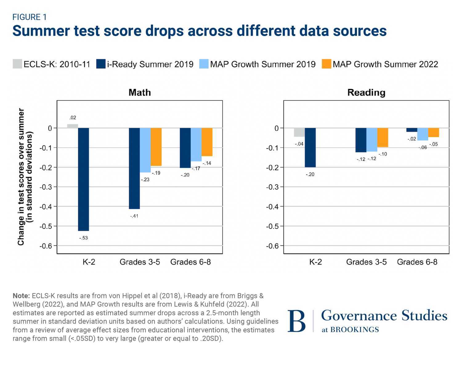
Read the zero line before comparing bar lengths. In the chart, a negative bar means the estimated fall score is lower than the spring score on that assessment’s scale. The small positive ECLS-K math estimate for grades K–2, about standard deviations, does not indicate a drop. The i-Ready math estimate for the same grade band, about , does. Neither bar shows the students’ total level of achievement: it shows an estimated change.
The assessments also give different-sized estimates. That variation matters, but the bars are not a contest in which the longest one automatically supplies the definitive summer effect. They come from different data sources. The next lesson will examine more closely how scales, test dates, and samples affect such comparisons. For now, the graph supports a narrower reading: depending on the assessment, measured summer performance may be roughly flat or may decline, with math drops often larger than reading drops in the estimates shown.
The slope during summer is not the whole-year result
A bar showing a spring-to-fall change gives two endpoints, but it does not show the rest of the year. A seasonal line graph adds that missing perspective. An upward line represents rising scores; a flatter upward line represents slower growth, not falling scores. A downward line represents a decline.
The following paper compares seasonal patterns in year-round and traditional-calendar schools. Concentrate on its graph and the explanation beside it, rather than on treating the comparison as a final verdict about calendar policy.
Year-Round School Calendars: Effects on Summer Learning ...
Read the paper’s explanation of how a calendar can change when measured learning occurs without necessarily changing the full-year gain.
In “Effects on summer and school-year learning,” go to the paragraph on the PDF page marked “Year-Round Schools--12.” Read from the sentence beginning “According to Table 2” through the explanation ending “according to Table 2”, then continue through the sentence beginning “Figure 1 summarizes the results graphically” and ending “stall out during the summer.” On the next page, marked “Year-Round Schools--13,” inspect both panels of Figure 1, “Learning in year-round and nine-month schools from the start of kindergarten to the end of first grade.” Follow each line from the leftmost date, Jun 98, to the rightmost date, May 00; stop at the legend beneath the panels. Compare the slopes during summer with those during the traditional school year.
In the paper’s Figure 1, the vertical axis is an ability score, not an amount of loss. Some plotted scores are negative because of how that scale is centered; a negative score is not the same thing as a negative change. The direction of each line between dates tells you whether measured performance rose, stayed level, or fell.
The paper reports a useful calendar contrast. Students on year-round calendars gained faster during summer, when their schedules included more school days. Students on nine-month calendars gained faster during the rest of the traditional school year, when their schedules included more school days. The year-round line’s summer advantage therefore did not imply a larger 12-month gain in this analysis. A seasonal advantage and a full-year advantage are different claims.
This also explains why “summer learning loss” needs precise wording. A graph can show that learning was slower than during school months even if its summer line still rises. Calling every slowdown a drop would misread the graph.
A group can lose ground without a gap widening
Now consider two groups rather than one. A claim about an achievement gap concerns the distance between their scores, not whether either group’s score fell.
Here is a deliberately simplified example on a common score scale:
| Group | Spring average | Fall average | Summer change |
|---|---|---|---|
| Higher-scoring group | 80 | 78 | |
| Lower-scoring group | 60 | 55 |
Both groups declined. The gap was 20 points in spring and 23 in fall, so it widened by 3 points. Had both groups declined by two points, their scores would still have fallen, but the gap would have remained 20 points.
More generally, if and are group averages on the same scale, the change in their gap is
The important comparison is between the groups’ changes. Two negative changes do not automatically produce a wider gap.
Return to the Brookings article for its comparison of schools grouped by poverty level.
Is summer learning loss real, and does it widen test score gaps by family income? | Brookings
Return to the Brookings article to compare an earlier claim about widening gaps with the more recent estimates plotted in Figure 2.
After Figure 1 and the paragraph discussing differences across assessments, find the paragraph beginning “A meta-analysis of summer learning studies.” Read from that paragraph through the Figure 2 explanation. Inspect Figure 2 directly below it, then stop before “Summary.” In each panel, compare the blue and orange bars for the same school level and summer; notice the uncertainty bars as well as the bar heights.
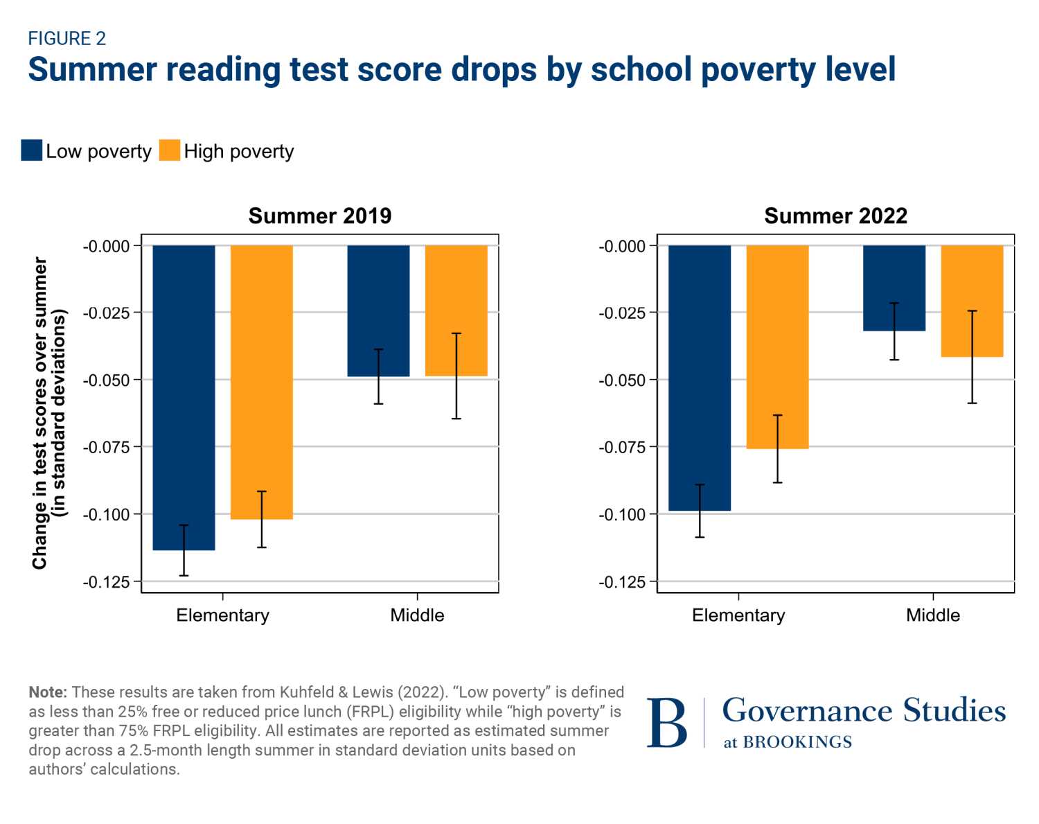
For example, in the 2022 elementary panel, both reading bars are below zero. The decline plotted for low-poverty schools is somewhat larger than the one plotted for high-poverty schools. Thus, the finding that both groups’ scores dropped is not evidence that the gap between these school groups widened. In the 2022 middle-school panel, the point estimates run slightly the other way, but the differences are small relative to the uncertainty shown. The article describes the declines for high-poverty schools as either statistically indistinguishable from, or less extreme than, those for low-poverty schools across these comparisons.
Two limits keep the interpretation disciplined. First, these categories describe school poverty levels, not a direct comparison of individual students sorted by family income. Second, bars showing changes do not show how large the groups’ score gap was in spring or fall. On a comparable scale, the difference between changes indicates the direction of a change in the gap; the bars alone do not reveal the gap’s starting size. Nor do these panels test whether a year-round calendar caused any of the patterns: they describe summer outcomes, not a calendar change.
Takeaways
When reading a seasonal achievement graph, check three separate things:
- Direction: Did the measured score rise, remain roughly flat, or fall?
- Rate: Was growth slower in summer than during school months, even if scores kept rising?
- Distance: Did the difference between two groups’ changes make their achievement gap wider, narrower, or roughly unchanged?
These distinctions prevent a summer decline from being mistaken for proof of a widening gap, or a summer advantage on one calendar from being mistaken for a full-year advantage. Next, the course will examine why test scales, testing dates, and student samples can change how credible a particular summer-loss estimate is.