Welcome to the first lesson in our module on Data Structures & Algorithms. In the previous module, we explored Java's Collections Framework, and you may recall we informally discussed the performance trade-offs between classes like ArrayList and LinkedList. For example, we noted that accessing an element in an ArrayList is very fast, while it's slow in a LinkedList.
In this lesson, we will formalize that notion of "fast" and "slow." We will learn how to analyze the efficiency of code using Big O notation. This is one of the most fundamental skills for a software engineer. It gives you a universal language to describe how an algorithm's performance changes as the amount of data it processes grows. Mastering this concept is absolutely critical for technical interviews and for writing scalable, professional-quality software.
Our goal is to understand what time and space complexity are, how to use Big O notation to express them, and how to analyze simple Java code to determine its complexity.
1. Why Do We Need Complexity Analysis?
You might wonder, "Why not just measure how long a program takes to run in seconds?" This seems intuitive, but it's not a reliable way to compare algorithms. The actual execution time depends heavily on factors that have nothing to do with the algorithm itself, such as the computer's processor speed, its memory, and what other programs are running.
The following video provides an excellent explanation of why we need a hardware-independent way to measure performance.
Time and Space Complexity - Strivers A2Z DSA Course
This video, "Time and Space Complexity," from the popular "Strivers A2Z DSA Course," explains the core motivation behind complexity analysis. The instructor's practical, interview-focused approach is highly relevant to your goals.
Watch from the beginning to understand why time taken in seconds is not a good measure of an algorithm's efficiency. Pay close attention to the Windows vs. MacBook example, which clearly illustrates how the same code can have different runtimes on different machines, while its fundamental efficiency (the rate of performance change) remains the same.
As the video explains, complexity analysis isn't about measuring exact time. Instead, it measures how the runtime (or memory usage) scales as the size of the input data, which we'll call n, increases.
- Time Complexity: Quantifies the amount of time an algorithm takes to run as a function of the input size
n. - Space Complexity: Quantifies the amount of memory an algorithm uses as a function of the input size
n.
2. Big O Notation: The Language of Efficiency
To express complexity, we use a mathematical notation called Big O notation. It looks like O(n), O(n^2), etc. Big O describes the upper bound or the worst-case scenario for an algorithm's complexity.
Why do we focus on the worst case? When building applications, we need to plan for the worst possible performance to ensure our system remains stable and responsive, even under heavy load. This guarantees that the performance will not be worse than what we've calculated. This is also what interviewers are almost always interested in.
The video below gives a great real-world analogy for why thinking about the worst-case is so important.
Time and Space Complexity | Big O Notation | DSA with JAVA Course
This video from "Jenny's Lectures CS IT" provides a clear introduction to time complexity and the reasoning behind focusing on the worst-case scenario.
Watch the segment from "why we consider worst case". The instructor's analogies, like planning for traffic during a major event, help build an intuitive understanding of this principle.
3. The Rules of Big O
To simplify complexity analysis, we follow a few standard rules. These rules help us focus on what's most important: how the algorithm behaves as the input size n becomes very large.
The "Strivers A2Z DSA Course" video breaks this down perfectly.
Time and Space Complexity - Strivers A2Z DSA Course
Let's return to the "Strivers A2Z DSA Course" video to learn the practical rules for calculating Big O.
Watch the segment that covers the three essential rules of Big O notation. The key rules explained here are: Always consider the worst-case scenario. Avoid (or drop) constants. For example, O(2n) simplifies to O(n). Avoid (or drop) lower-order terms. For example, O(n^2 + n) simplifies to O(n^2). The video provides clear reasoning for each rule, emphasizing that for large inputs, the constants and lower-order terms become insignificant compared to the dominant term.
4. Common Complexity Classes
Algorithms are categorized into different "complexity classes" based on their Big O notation. Let's explore the most common ones, from most efficient to least efficient. The following article provides an excellent, math-free overview with diagrams and Java examples.
Big O Notation and Time Complexity – Easily Explained
This article from HappyCoders.eu is a fantastic, practical guide to understanding the most common complexity classes. It uses code and graphs instead of formal math proofs.
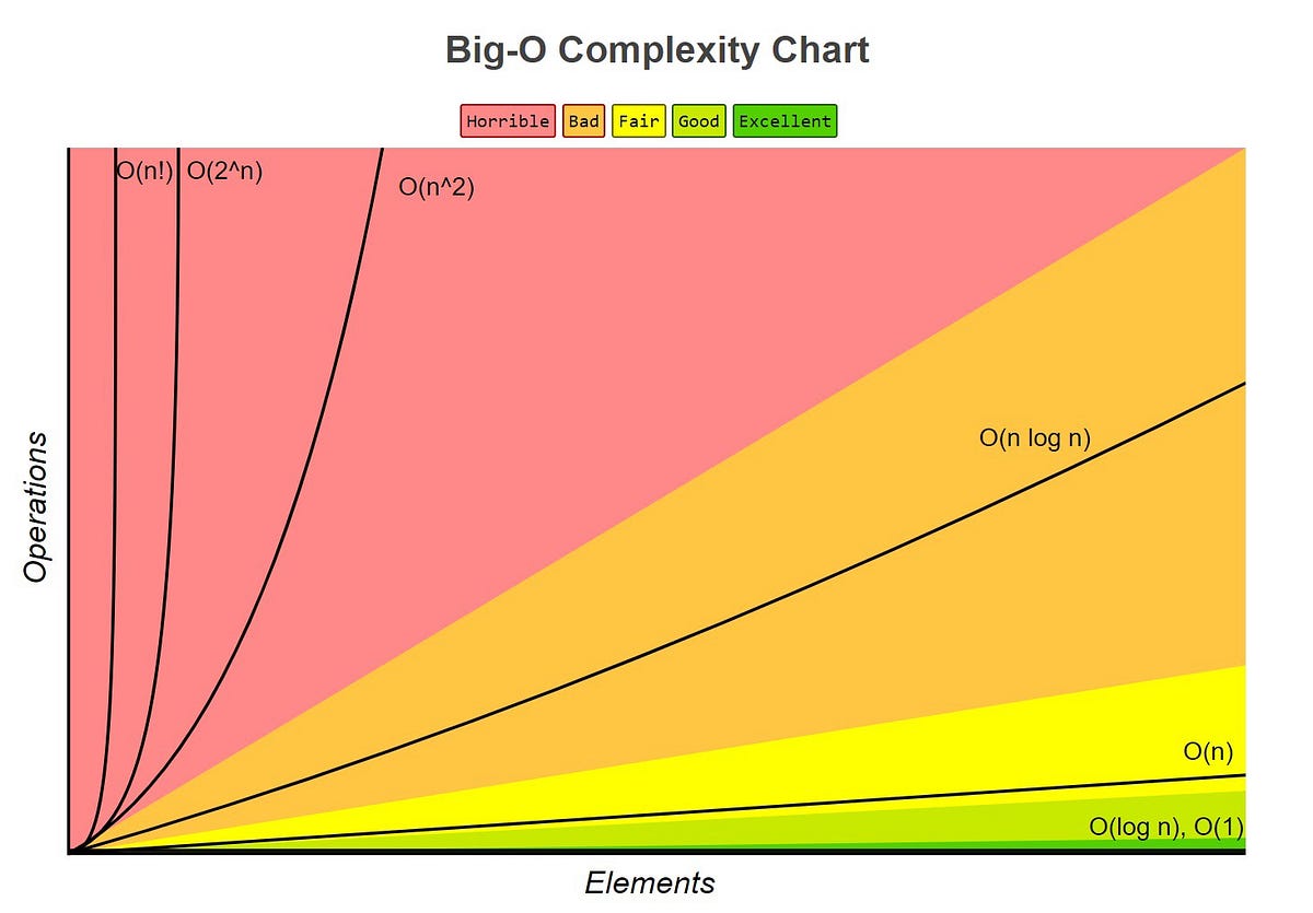
Please read through the article, focusing on the following sections: Start with the introductory sections on Types of Complexity and Complexity Classes to get the basic definitions. Then, read the detailed explanations for each of the following classes: O(1) – Constant Time: Read the full section. O(n) – Linear Time: Read the full section. O(n²) – Quadratic Time: Read the full section. O(log n) – Logarithmic Time: Read the full section. O(n log n) – Quasilinear Time: Read the full section. Finally, read the summary sections that compare these classes and briefly mention others like O(2^n) and O(n!). Pay close attention to the graphs that visually compare the growth rates.
To help you visualize these growth rates, here is a classic chart.
5. Analyzing Simple Java Code
Now, let's apply these concepts to analyze some actual Java code. The key is to count the number of operations relative to the input size n, keeping the rules of Big O in mind. Loops are the primary factor that increases complexity.
The video from "Strivers A2Z DSA Course" has a great segment where the instructor analyzes a few common loop structures.
Time and Space Complexity - Strivers A2Z DSA Course
Let's watch how to apply Big O analysis to code.
Watch the examples starting at this timestamp. The instructor analyzes two key patterns: A nested for loop where both loops run n times. This results in n * n = n^2 operations, giving a complexity of O(n^2). A nested for loop where the inner loop's iterations depend on the outer loop (e.g., for i=0 to n, for j=0 to i). This still results in a complexity of O(n^2). The sum 1 + 2 + ... + n is n*(n+1)/2, which simplifies to O(n^2).
Here's a quick summary of how to analyze loops:
- A single loop that iterates from
0tonisO(n). - Two separate, sequential loops that each iterate to
nareO(n) + O(n), which simplifies toO(n). - A loop nested inside another loop, where both iterate to
n, isO(n * n)orO(n^2).
6. What About Space Complexity?
So far, we've focused on time. Space complexity follows the same Big O principles, but it measures memory usage instead of operations.
A key distinction to understand is input space vs. auxiliary space.
- Input Space: The memory used to store the input data itself (e.g., the array you are given).
- Auxiliary Space: The extra or temporary space your algorithm uses to solve the problem.
In interviews, when someone asks for "space complexity," they usually mean the auxiliary space complexity.
Let's read a formal definition.
This article from GeeksForGeeks provides clear definitions for space complexity and auxiliary space.
Please read the sections titled "Space Complexity" and the explanation of auxiliary space. Note the examples for O(1) space (adding two numbers) and O(N) space (creating a frequency map/dictionary).
A crucial piece of practical advice for interviews comes from the "Strivers A2Z DSA Course" video.
Time and Space Complexity - Strivers A2Z DSA Course
This segment discusses an important professional best practice related to space complexity.
Watch the section on space complexity, particularly the advice about not modifying the input data, starting at this timestamp. While modifying an input array might save space (leading to O(1) auxiliary space), it's generally considered bad practice. In a real-world application, other parts of the system might still need the original, unmodified data. It's almost always better to use extra space (O(n)) to create a copy and work on that instead.
7. Putting It All Together: A Practical Reference
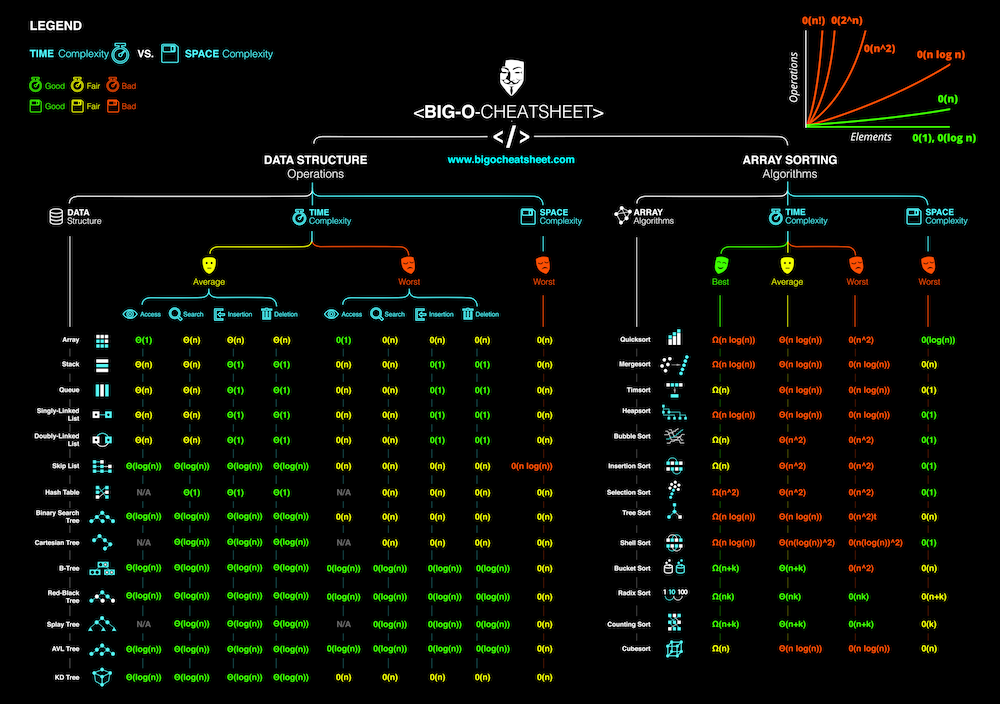
You now have the foundational knowledge to analyze algorithm complexity. The image below is a famous "cheat sheet" that summarizes the time and space complexity for common operations on various data structures and sorting algorithms. We will cover many of these in upcoming lessons.
For now, look at the "Data Structure Operations" section. Can you see the complexities we discussed for Array, ArrayList (Dynamic Array in some contexts), and HashMap (Hash Table)? This is the formal representation of the performance characteristics we've been talking about.
Conclusion
In this lesson, we established a formal framework for analyzing algorithm efficiency. This is a skill you will use throughout your career as a software engineer.
Here are the key takeaways:
- Complexity analysis measures how an algorithm's runtime or space usage scales with the input size
n. - Big O notation is used to express the worst-case complexity, which provides a performance guarantee.
- When calculating Big O, we drop constants and non-dominant terms to focus on the growth rate for large inputs.
- The most common complexity classes you'll encounter are
O(1),O(log n),O(n),O(n log n), andO(n^2). - Space complexity typically refers to the auxiliary space—the extra memory an algorithm uses, not including the input itself.
In our next lesson, we will put this theory into practice. We will implement two search algorithms, linear search and binary search, and analyze them to see a direct comparison between an O(n) algorithm and a much more efficient O(log n) algorithm.