Confidence Intervals: Precision and Sample Size

1. From Point Estimate to a Range of Confidence

In the last lesson, we calculated a sample mean, $\bar{x}$, as our best single guess for the population mean, $\mu$. This is called a point estimate. But we know that if we took a different sample, we'd get a different $\bar{x}$. A confidence interval accounts for this sampling variability by providing a range around our point estimate.

To get a clear introduction to this idea, let's watch a short, conceptual video.

As the video explained, a confidence interval is constructed from two key components:

• Point Estimate: The sample statistic (e.g., the sample mean), which forms the center of the interval.
• Margin of Error: The "plus or minus" value that is added to and subtracted from the point estimate to create the range. The formula is:
  $\text{Confidence Interval}=\text{Point Estimate}\pm \text{Margin of Error}$

The video also highlighted the two factors that influence the margin of error, and thus the width of the interval:

1. Variation in the population: More variability in the underlying data leads to a wider interval (more uncertainty).
2. Sample size: This is a factor we can often control, and it has a direct impact on our confidence. We'll dive deeper into this relationship shortly.

2. The Correct Way to Interpret a Confidence Interval

This is one of the most misunderstood concepts in introductory statistics, so let's be very precise. A confidence interval comes with a confidence level, most commonly 95%.

A common mistake is to say: "There is a 95% probability that the true population mean falls within this specific interval." This is incorrect. The true population parameter $\mu$ is a fixed value; it's either in our calculated interval or it isn't. The probability is 1 or 0, we just don't know which.

The 95% confidence is about the reliability of the method, not a single outcome.

For a detailed explanation of this crucial point, please read the following section from an excellent article on Medium.

To summarize the key idea from the article:

The correct interpretation: If we were to draw many random samples from the same population and construct a 95% confidence interval for each sample, we would expect about 95% of those intervals to capture the true population parameter.

To make this abstract idea concrete, let's watch a simulation. The following video segment plots 25 different confidence intervals calculated from 25 different samples taken from the same population.

This visualization perfectly illustrates the frequentist interpretation: any one interval might miss the true parameter, but the method ensures that over the long run, the stated percentage of intervals will be successful.

3. The Power of Sample Size

As we saw in the first video, sample size has a major impact on the width of the confidence interval. Let's make this relationship explicit.

The margin of error for a confidence interval for a mean is typically calculated as:

Where $n$ is the sample size. The critical value comes from a Z- or t-distribution and depends on the confidence level. You don't need to memorize this formula right now, but notice where $n$ is: in the denominator, under a square root.

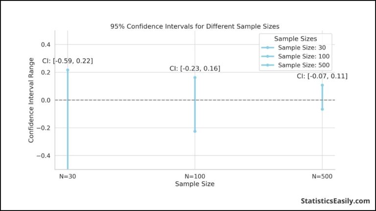
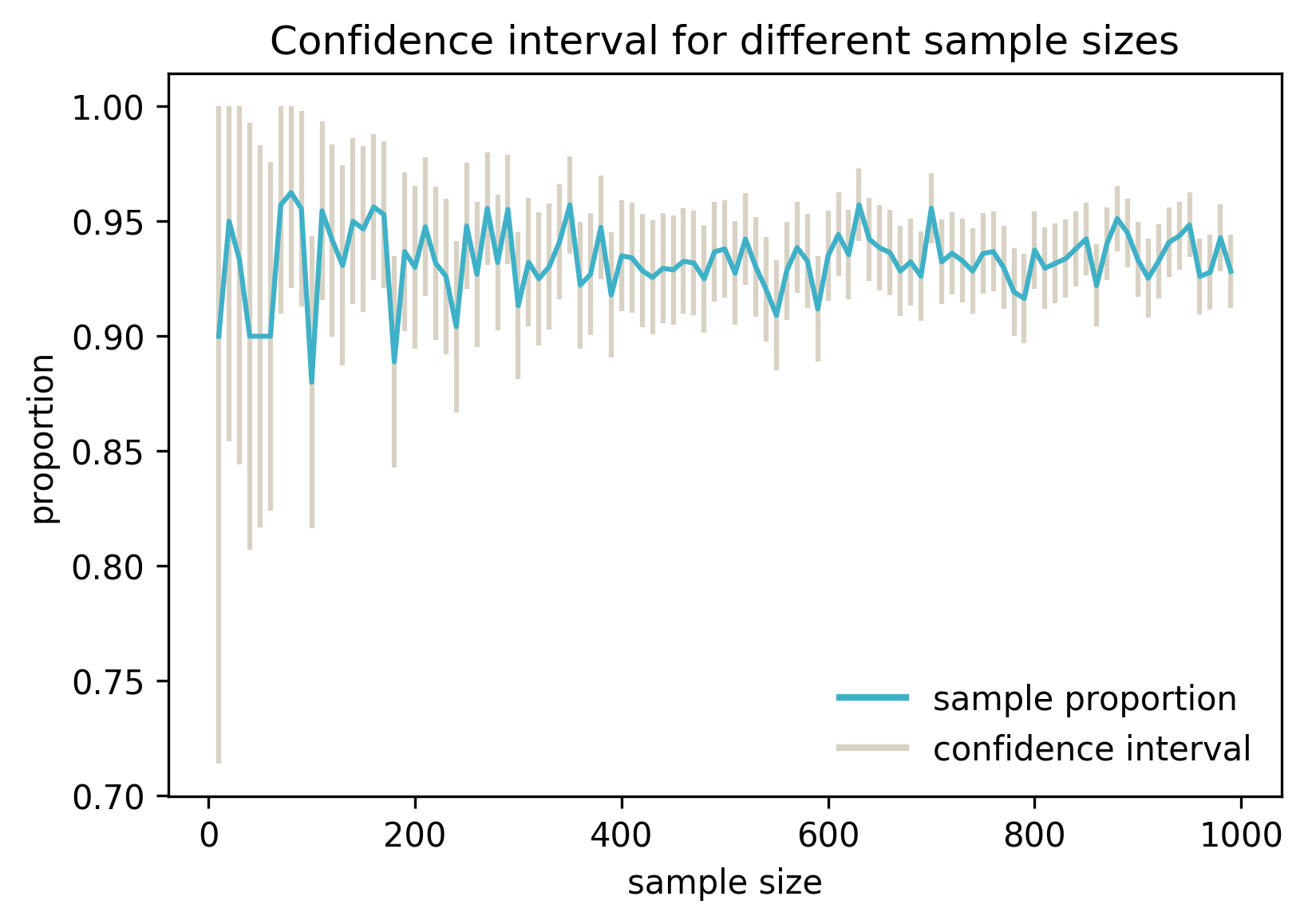
This means that as the sample size $n$ increases, the margin of error decreases, resulting in a narrower, more precise confidence interval. Intuitively, this makes sense: the more data we have, the more certain we are about our estimate of the population parameter.

These images show this effect clearly.

4. Calculating a Confidence Interval in Python

Now let's bridge theory and practice. While it's important to understand the concepts, in your daily work as a data scientist, you'll use libraries to do the calculations. The scipy.stats module is the standard tool for this in Python.

Let's walk through an example from the Medium article we read earlier, which calculates the 95% confidence interval for the mean sepal length of the Iris setosa flower species.

The code in the article calculates the interval manually. However, scipy provides a more direct way to do this using the stats.t.interval() function, which is what you'd typically use.

Here's how you would do it for the same Iris data, combining the steps into a more streamlined process:

import numpy as np
import pandas as pd
from scipy import stats
import seaborn as sns




# Load the Iris dataset
iris = sns.load_dataset('iris')
setosa_sepal_length = iris[iris['species'] == 'setosa']['sepal_length']




# --- Calculate the 95% confidence interval ---




# 1. Define confidence level
confidence_level = 0.95




# 2. Calculate degrees of freedom (sample size - 1)
degrees_freedom = len(setosa_sepal_length) - 1




# 3. Calculate sample mean and standard error
sample_mean = np.mean(setosa_sepal_length)
standard_error = stats.sem(setosa_sepal_length) # sem = standard error of the mean




# 4. Use scipy to calculate the interval
confidence_interval = stats.t.interval(alpha=confidence_level, 
                                       df=degrees_freedom, 
                                       loc=sample_mean, 
                                       scale=standard_error)

print(f"Sample Mean: {sample_mean:.2f}")
print(f"95% Confidence Interval: ({confidence_interval[0]:.2f}, {confidence_interval[1]:.2f})")




# Output:
# Sample Mean: 5.01
# 95% Confidence Interval: (4.91, 5.10)

Interpretation: Based on our sample, we are 95% confident that the true population mean for the sepal length of all Iris setosa flowers lies between 4.91 cm and 5.10 cm.

Conclusion

Excellent work today! We've taken a major step from simple point estimates to a more nuanced and powerful way of expressing statistical findings.

Here are your key takeaways:

• A confidence interval provides a range of plausible values for an unknown population parameter, based on a sample.
• The confidence level (e.g., 95%) refers to the long-term success rate of the method, not the probability that one specific interval contains the true parameter.
• The width of a confidence interval reflects the precision of our estimate.
• Increasing the sample size is the most direct way to decrease the margin of error and obtain a narrower, more precise confidence interval.
• In practice, we use libraries like scipy.stats in Python to calculate confidence intervals efficiently.

Preview of the next lesson:

Confidence intervals and hypothesis tests are two sides of the same coin. A confidence interval asks, "What is the range of plausible values for a parameter?" A hypothesis test asks a more direct yes/no question, like "Is it plausible that the parameter is equal to zero?" In our next lesson, we will learn how to perform and interpret one of the most common hypothesis tests: the t-test, which is used to compare the means of two groups.