T-Tests in Python: Comparing Group Means

1. The Core Idea: Hypothesis, Evidence, and P-Values

At its heart, a hypothesis test is a formal way to decide if an observed difference is real or just a fluke of random chance. Imagine you run an A/B test for a new website button. The new button (B) gets a slightly higher click-through rate than the old one (A). A t-test helps you determine if that improvement is statistically significant or if you just got lucky with the users you happened to show it to.

To do this, we set up two competing hypotheses:

• Null Hypothesis ($H_0$): This is the default, skeptical assumption. It states there is no difference between the groups. Any observed difference is due to random sampling variation. (e.g., "The new button has no effect on the click-through rate.")
• Alternative Hypothesis ($H_a$): This is what we are trying to find evidence for. It states there is a real difference between the groups. (e.g., "The new button changes the click-through rate.")

The t-test then calculates a p-value. The p-value is the probability of seeing a difference as large as the one you observed if the null hypothesis were true.

• A small p-value (typically < 0.05) suggests that your observed result is very unlikely under the null hypothesis. This gives you evidence to reject the null hypothesis in favor of the alternative.
• A large p-value (typically ≥ 0.05) suggests that your result is quite plausible under the null hypothesis. You fail to reject the null hypothesis due to lack of evidence.

To get a more intuitive feel for this, please watch the first part of this short video.

2. The Three Flavors of T-Tests

Not all comparisons are the same. Depending on your data and the question you're asking, you'll need one of three main types of t-tests.

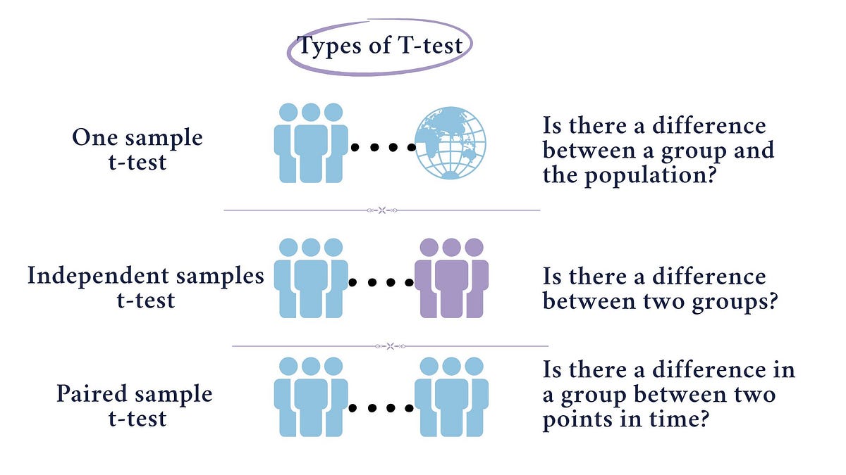
Here's a breakdown:

1. Independent Samples T-Test: This is the most common type. Use it when you are comparing the means of two separate, independent groups.

   • Example: Comparing the average purchase amount of customers who received a discount (group A) versus those who did not (group B).

2. Paired Samples T-Test: Use this when you are comparing the means of the same group at two different points in time or under two different conditions. The samples are "paired" because each data point in the first group is directly related to one in the second.

   • Example: Measuring the weight of the same group of people before and after a diet program.

3. One-Sample T-Test: Use this when you are comparing the mean of a single group to a known or hypothesized value.

   • Example: Testing if the average IQ score of a class of students is significantly different from the national average of 100.

3. T-Tests in Practice with Python

Now, let's get our hands dirty. The scipy.stats library is your go-to tool for statistical tests in Python. We'll watch a video that demonstrates how to perform all three types of t-tests, and I'll provide the code for you to run and experiment with.

One-Sample T-Test (ttest_1samp)

As shown in the video, we use stats.ttest_1samp() to compare the mean of a single sample to a known population mean.

Here's the code from the video. Run it in your own notebook.

import numpy as np
from scipy import stats




# Generate some dummy data
# We are creating a population with a mean age of ~43
population_ages = stats.poisson.rvs(loc=18, mu=35, size=1500)
population_mean = np.mean(population_ages)




# Now, let's take a sample from a slightly different distribution (mean age ~38)
minnesota_ages = stats.poisson.rvs(loc=18, mu=30, size=50)
sample_mean = np.mean(minnesota_ages)

print(f"Population Mean: {population_mean:.2f}")
print(f"Sample Mean: {sample_mean:.2f}")




# Perform the one-sample t-test
t_statistic, p_value = stats.ttest_1samp(a=minnesota_ages, popmean=population_mean)

print(f"\nT-statistic: {t_statistic:.4f}")
print(f"P-value: {p_value:.4f}")




# Interpretation
if p_value < 0.05:
    print("\nThe p-value is less than 0.05. We reject the null hypothesis.")
    print("Conclusion: The sample mean is significantly different from the population mean.")
else:
    print("\nThe p-value is not less than 0.05. We fail to reject the null hypothesis.")
    print("Conclusion: There is not enough evidence to say the sample mean is different from the population mean.")

The output shows a small p-value, leading us to conclude that our sample of Minnesota voters is, on average, significantly different in age from the general population.

Now, let's continue with the video for the independent and paired t-tests.

Independent Samples T-Test (ttest_ind)

This test compares two independent groups. Here's the code to compare the minnesota_ages sample with a new wisconsin_ages sample.

# Generate a second sample for Wisconsin, with a slightly different mean
wisconsin_ages = stats.poisson.rvs(loc=18, mu=33, size=50)
print(f"Minnesota Mean Age: {np.mean(minnesota_ages):.2f}")
print(f"Wisconsin Mean Age: {np.mean(wisconsin_ages):.2f}")




# Perform the independent samples t-test
t_statistic, p_value = stats.ttest_ind(a=minnesota_ages, b=wisconsin_ages, equal_var=False)



# We set equal_var=False because we don't know if the two samples have the same variance. This runs a Welch's t-test, which is generally more reliable.

print(f"\nT-statistic: {t_statistic:.4f}")
print(f"P-value: {p_value:.4f}")

if p_value < 0.05:
    print("\nConclusion: The mean ages of the two groups are significantly different.")
else:
    print("\nConclusion: There is not enough evidence to say the mean ages are different.")

Paired Samples T-Test (ttest_rel)

This test is for related samples, like "before" and "after" measurements on the same subjects.

# Generate data for a 'before' and 'after' scenario
np.random.seed(0) # for reproducibility
before_treatment = stats.norm.rvs(loc=70, scale=10, size=20)



# after treatment, there's a small decrease in values on average
after_treatment = before_treatment - np.random.normal(loc=1.5, scale=3, size=20)

print(f"Mean Before: {np.mean(before_treatment):.2f}")
print(f"Mean After: {np.mean(after_treatment):.2f}")




# Perform the paired samples t-test
t_statistic, p_value = stats.ttest_rel(a=before_treatment, b=after_treatment)

print(f"\nT-statistic: {t_statistic:.4f}")
print(f"P-value: {p_value:.4f}")

if p_value < 0.05:
    print("\nConclusion: There is a significant difference between the 'before' and 'after' measurements.")
else:
    print("\nConclusion: There is not a significant difference between the measurements.")

4. Beyond the P-Value: Errors and Assumptions

Just getting a p-value isn't the end of the story. It's crucial to understand the potential for errors and the assumptions your test relies on.

Type I and Type II Errors

When we make a decision based on a p-value, we can sometimes be wrong. There are two types of errors:

• Type I Error (False Positive): You reject the null hypothesis when it's actually true. You conclude there is a difference, but there isn't one. The probability of this error is equal to your significance level ($\alpha$), which is why we choose a small value like 0.05.
• Type II Error (False Negative): You fail to reject the null hypothesis when it's actually false. There really is a difference, but your test failed to detect it.

This final video segment explains this trade-off clearly.

Assumptions of the T-Test

For the results of a t-test to be reliable, the data should meet a few key assumptions. While we won't go deep into testing them today, it's vital to know what they are:

1. Independence: The observations in one group should be independent of the observations in the other group (for an independent t-test).
2. Normality: The data in each group should be approximately normally distributed. T-tests are fairly robust to violations of this, especially with larger sample sizes (n > 30).
3. Homogeneity of Variances: The two groups should have approximately equal variances. (Using equal_var=False in ttest_ind helps relax this assumption).

For a quick reference on these assumptions and how to check them in Python, you can review the following article.

Conclusion

Great job today! You've just learned one of the most widely used statistical tools in data science. It's a cornerstone of experimental analysis and will serve you well in many projects.

Here are your key takeaways:

• A t-test is a hypothesis test used to compare the means of one or two groups.
• It works by comparing the null hypothesis (no difference) with the alternative hypothesis (there is a difference).
• The p-value tells you the probability of observing your data if the null hypothesis were true. A small p-value (< 0.05) is evidence against the null hypothesis.
• There are three main types: one-sample, independent samples, and paired samples, each for a different experimental design.
• You can easily perform these tests in Python using the scipy.stats module with ttest_1samp, ttest_ind, and ttest_rel.

Preview of the next lesson:

The t-test is a classic example of frequentist statistics, where we make decisions based on the frequency of data occurring in the long run. However, there's another major school of thought in statistics: the Bayesian approach. In our next lesson, we will dive into Bayes' theorem and learn how it allows us to update our beliefs about a hypothesis as we gather new evidence. This provides a powerful and often more intuitive framework for reasoning under uncertainty.