Correlation vs. Causation: Unpacking Relationships

1. What is Correlation?

In data science, we are constantly looking for relationships between variables. Does more advertising spending lead to more sales? Is a student's study time related to their exam score? Correlation gives us a way to numerically measure the statistical relationship between two variables.

A correlation can be:

• Positive: When one variable increases, the other tends to increase. (e.g., height and weight).
• Negative: When one variable increases, the other tends to decrease. (e.g., car speed and travel time).
• Weak or No Correlation: The variables don't seem to be related in any clear way.

The best way to get an initial feel for correlation is to visualize it. Scatter plots are perfect for this.

To start, let's read a short introductory text that defines correlation and shows these different types visually.

The number that quantifies the strength and direction of this relationship is called the correlation coefficient.

2. Measuring Linear Relationships: Pearson's 'r'

The most common type of correlation coefficient is the Pearson correlation coefficient, denoted by $r$. It measures the strength and direction of a linear relationship between two variables.

Its value always falls between -1 and +1:

• $r=+1$: Perfect positive linear relationship.
• $r=-1$: Perfect negative linear relationship.
• $r=0$: No linear relationship.

Values between 0 and 1 indicate a positive correlation, and values between -1 and 0 indicate a negative correlation. The closer the value is to 1 or -1, the stronger the linear relationship.

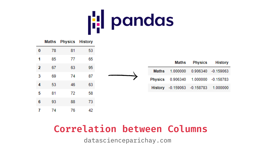
In your practical work as a data scientist, you'll most often calculate this using pandas. Given a DataFrame, the .corr() method computes the pairwise correlation between all numerical columns.

Here's how you'd do it in Python. Let's create a DataFrame and calculate the Pearson correlation matrix.

import pandas as pd
import numpy as np




# Create a sample DataFrame
data = {
    'study_hours': [2, 3, 5, 1, 6, 4, 7],
    'exam_score': [65, 70, 85, 60, 90, 75, 95],
    'sleep_hours': [8, 7, 6, 9, 5, 7, 6]
}
df = pd.DataFrame(data)




# Calculate the Pearson correlation matrix
# By default, method is 'pearson'
correlation_matrix = df.corr()

print(correlation_matrix)

Your Turn: Run the code above. What can you conclude about the relationship between study_hours and exam_score? What about study_hours and sleep_hours?

You should see a strong positive correlation between study_hours and exam_score (close to +1) and a strong negative correlation between study_hours and sleep_hours (close to -1).

3. Beyond Linearity: Spearman's 'rho' (ρ)

Pearson's coefficient is great, but it has a limitation: it only captures linear relationships. What if a relationship is consistent but not a straight line?

This is where the Spearman rank correlation coefficient, denoted by rho ($\rho$), comes in. As we touched on in the last lesson, this is a non-parametric measure. It doesn't use the raw data values but instead uses their ranks. Because of this, Spearman's coefficient can measure any monotonic relationship—one where the variables consistently move in the same or opposite directions, but not necessarily at a constant rate.

The following video does an excellent job of visually explaining the difference.

Because it uses ranks, Spearman's correlation is also less sensitive to outliers than Pearson's.

Calculating Spearman's correlation in pandas is just as easy. You simply specify method='spearman' in the .corr() function.

# Create data with a non-linear but monotonic relationship
data_nonlinear = {
    'x': [1, 2, 3, 4, 5, 6, 7, 8],
    'y_linear': [2, 4, 6, 8, 10, 12, 14, 16], # Perfectly linear
    'y_monotonic': [1, 4, 9, 16, 25, 36, 49, 64] # y = x^2, monotonic but not linear
}
df_nonlinear = pd.DataFrame(data_nonlinear)




# Calculate both Pearson and Spearman correlations
pearson_corr = df_nonlinear.corr(method='pearson')
spearman_corr = df_nonlinear.corr(method='spearman')

print("--- Pearson Correlation ---")
print(pearson_corr)
print("\n--- Spearman Correlation ---")
print(spearman_corr)

Run this code. Notice that for the relationship between x and y_monotonic, Spearman's correlation is a perfect 1, while Pearson's is slightly lower because the relationship isn't a straight line. This demonstrates the practical difference and why choosing the right coefficient matters.

4. The Golden Rule: Correlation Is Not Causation

This is arguably the most important concept in this entire module. Just because two variables are strongly correlated does not mean that one causes the other.

This is a common trap for junior analysts and is frequently misrepresented in news headlines. A correlation can appear for several reasons:

1. Causation: One variable actually causes the other (e.g., more rainfall causes higher river levels).
2. Confounding Variable: A hidden third variable is causing both. This is the most common source of confusion.
3. Coincidence: In large datasets, you can find variables that are correlated just by random chance.

Let's watch a video that brings this point to life with clear, memorable examples.

The video makes the point perfectly. The correlation between ice cream sales and shark attacks isn't because ice cream makes sharks attack. The confounding variable is hot weather, which causes more people to buy ice cream and causes more people to go swimming.

To formalize this, here are the key pitfalls to be aware of:

• Third Variable Problem: An unobserved variable, Z, causes both X and Y, creating a spurious correlation between them. (e.g., Temperature causing both ice cream sales and shark attacks).
• Directionality Problem: We know X and Y are correlated, but we don't know if X causes Y or if Y causes X. (e.g., Does watching violent TV make people aggressive, or do aggressive people choose to watch violent TV?).

Distinguishing correlation from causation is one of the hardest problems in data science. The most reliable way to establish causation is through a randomized controlled trial (RCT), where you actively intervene and change one variable to see its effect on another. Since that's often not possible, we rely on careful analysis, domain knowledge, and a healthy dose of skepticism.

Conclusion

Fantastic job today! You've learned how to quantify relationships in your data and, more importantly, how to interpret those findings with the caution and rigor of a true data scientist.

Key Takeaways:

• Correlation coefficients (r and $\rho$) measure the strength and direction of a relationship, ranging from -1 to +1.
• Pearson's r is for measuring linear relationships and is sensitive to outliers.
• Spearman's $\rho$ is for measuring monotonic relationships and is more robust to non-linearity and outliers.
• Both are easily calculated in pandas using df.corr(method='...').
• The Golden Rule: Correlation does not imply causation. Always be critical of observed relationships and consider potential confounding variables.

Preview of the next module:

This lesson concludes our module on strengthening your statistical foundations. You are now equipped with key concepts like hypothesis testing, Bayesian updates, and correlation analysis.

These tools are essential for Exploratory Data Analysis (EDA), which is the process of "getting to know" your data. In our next module, we will officially begin our journey into practical EDA. Our first lesson will focus on how to compute and interpret summary statistics, the very first step in characterizing any new dataset you encounter.