Summarizing Data Distributions

1. The Big Picture: A First Glance at Your Data

When you first load a dataset into a pandas DataFrame, your initial goal is to get a quick, high-level summary. You want to answer questions like:

• How many data points are there?
• What's the average value?
• What are the minimum and maximum values?

Pandas provides a wonderfully efficient method for this: .describe(). It calculates several key descriptive statistics for all numerical columns in your DataFrame at once.

To see it in action, let's watch a short segment from a video by Rob Mulla.

As you saw, a single command gives you a wealth of information. Let's try it ourselves. Imagine we have a dataset of house prices.

import pandas as pd
import numpy as np




# Sample data representing house prices in thousands of dollars
data = {'price_k': [150, 155, 160, 175, 180, 185, 185, 190, 210, 220, 250, 450]}
df = pd.DataFrame(data)




# Get the descriptive statistics
description = df['price_k'].describe()
print(description)

Your Turn: Run this code. The output of .describe() gives you:

• count: The number of non-missing values.
• mean: The arithmetic average.
• std: The standard deviation (we'll cover this shortly).
• min: The minimum value.
• 25%, 50%, 75%: The quartiles (or percentiles), where the 50th percentile is the median.
• max: The maximum value.

Look at the mean (205.0) and the median (50%, which is 185.0). Why are they different? And what does the max value of 450 tell us? The .describe() output gives us clues, but to truly interpret them, we need to understand each component.

2. Measures of Central Tendency: What's a "Typical" Value?

Measures of central tendency aim to identify the center or "typical" value of a distribution. The three most important are the mean, median, and mode.

• Mean: The average value. Highly sensitive to outliers (extreme values).
• Median: The middle value of a sorted dataset. It's robust to outliers.
• Mode: The most frequently occurring value. Useful for categorical data or discrete numerical data with repeated values.

The following video provides an excellent explanation of these concepts and, crucially, demonstrates why the choice between mean and median matters so much in practice.

The relationship between the mean and median tells you about the symmetry of your data.

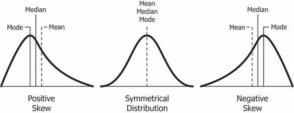
For our house price data, the mean (205k) is higher than the median (185k). This indicates a right-skewed distribution, likely caused by a few very expensive houses (like the one priced at 450k) pulling the average up. In this case, the median is a better measure of the "typical" house price because it's less affected by that one outlier.

3. Measures of Dispersion: How Spread Out is the Data?

Knowing the center isn't enough. Two datasets can have the same mean but be vastly different. We also need to measure the dispersion or spread of the data.

Key measures of spread include:

• Range: The difference between the maximum and minimum values. Simple, but very sensitive to outliers.
• Variance: The average of the squared differences from the Mean. Its units are squared (e.g., dollars-squared), making it hard to interpret directly.
• Standard Deviation ($\sigma$): The square root of the variance. It's the most common measure of spread and is in the same units as the data. It tells you, on average, how far each point is from the mean. Like the mean, it's sensitive to outliers.
• Interquartile Range (IQR): The range of the middle 50% of the data (i.e., the distance between the 75th and 25th percentiles). Since it focuses on the middle of the data, it is robust to outliers.

Let's return to the same video to see how these are calculated and interpreted.

In our house price example, the standard deviation is about 87.6k. This is a large number relative to the median, confirming that the prices are very spread out. The IQR would be Q3 - Q1, or 215k - 177.5k = 37.5k. This much smaller number tells us that the central 50% of houses are clustered within a 37.5k price range, confirming our suspicion that the high overall spread is driven by outliers.

4. Measures of Shape: Skewness and Kurtosis

Finally, we can describe the shape of the distribution with two more statistics:

• Skewness: Measures the asymmetry of the distribution.
  • Positive Skew (Right-skewed): Long tail to the right (like our house prices). Skewness > 0.
  • Negative Skew (Left-skewed): Long tail to the left. Skewness < 0.
  • Symmetrical: Skewness ≈ 0.
• Kurtosis: Measures the "tailedness" of the distribution. It tells you how much of the data is in the tails versus the center.
  • High Kurtosis (Leptokurtic): Heavy tails and a sharp peak, meaning more outliers.
  • Low Kurtosis (Platykurtic): Light tails and a flatter peak, meaning fewer outliers.

Let's watch the final segment of the video to see how these are calculated.

5. Hands-On Practice: Synthesizing Your Knowledge

Now it's time to apply everything we've learned to a real dataset. You're going to use the Wisconsin Breast Cancer dataset, a classic dataset in machine learning. Your goal is to compute and interpret summary statistics to understand its features.

The following resource provides a complete walkthrough with code. Your task is to work through it, run the code, and focus on interpreting the output.

By completing this exercise, you've moved from just knowing the definitions to actively using these statistics to explore data and generate initial hypotheses—the very essence of EDA.

Conclusion

Excellent work! You have just taken the first and most fundamental step in any data analysis project. Characterizing distributions with summary statistics is the bedrock upon which all further analysis—and visualization—is built.

Key Takeaways:

• Descriptive statistics are used to summarize data through measures of central tendency (mean, median, mode), dispersion (standard deviation, IQR), and shape (skewness, kurtosis).
• The pandas df.describe() method is your best friend for a quick, comprehensive overview.
• The choice of statistic matters: median and IQR are robust to outliers, while mean and standard deviation are sensitive to them. Comparing them gives clues about the data's distribution.
• You can compute these statistics for the whole dataset or for specific groups to find patterns and differences.

Preview of the next lesson:

Numbers are powerful, but a picture is worth a thousand words. Now that you know how to describe distributions numerically, our next lesson will focus on visualizing them. We will learn to create and interpret histograms, box plots, and scatter plots, which will bring the insights you've uncovered today to life.