Data Visualization with Matplotlib and Seaborn

1. Visualizing a Single Variable: The Histogram

In the last lesson, you learned that statistics like skewness can tell you if a distribution is lopsided. A histogram is the visual proof. It shows the distribution of a single numerical variable by grouping data into "bins" and plotting the frequency of data points in each bin.

Let's start by understanding the basics of creating a histogram with matplotlib, the foundational plotting library in Python.

Now, let's see a practical demonstration using pandas, which uses matplotlib under the hood. We'll also see a related plot type, the Kernel Density Estimate (KDE), which provides a smoothed version of the histogram.

Interpreting a Histogram

When you look at a histogram, you are looking for the story of that variable. Ask yourself:

• Shape: Is the distribution symmetric (like a bell curve), right-skewed (long tail to the right), or left-skewed? This visually confirms the skewness statistic you learned about.
• Modality: How many peaks does it have? One peak is "unimodal," two is "bimodal." Multiple peaks might suggest there are distinct subgroups in your data.
• Center: Where is the center of the distribution? You can visually estimate the mean or median.
• Spread: Are the values tightly clustered or widely spread out?

While matplotlib is powerful, the seaborn library simplifies the creation of statistically-informed and aesthetically pleasing plots. Here's how you'd create a histogram with seaborn, which also makes it easy to overlay that smooth KDE curve.

import seaborn as sns
import matplotlib.pyplot as plt
import pandas as pd




# Using the same breast cancer dataset from the last lesson
# You can download it here: https://www.kaggle.com/datasets/uciml/breast-cancer-wisconsin-data
df = pd.read_csv('data.csv') 




# Create a histogram of the 'radius_mean' feature with a KDE overlay
sns.histplot(data=df, x='radius_mean', kde=True)
plt.title('Distribution of Mean Radius')
plt.xlabel('Mean Radius')
plt.ylabel('Frequency')
plt.show()

Run this code. You'll notice the seaborn plot is not only visually appealing but also combines the binned frequency (histogram) with a smooth density estimate (KDE), giving a very complete picture of the distribution in a single line of code.

2. Summarizing a Distribution: The Box Plot

The box plot is a compact and powerful visualization. It directly corresponds to the five-number summary you got from the df.describe() method in our last lesson: minimum, first quartile (Q1), median (Q2), third quartile (Q3), and maximum.

Its real power lies in showing spread and identifying potential outliers in a very clean format.

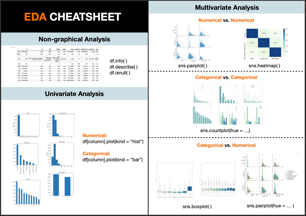
Let's review the anatomy of a box plot and see how to create one.

The true strength of box plots in EDA comes from comparing distributions. With seaborn, this is incredibly easy. Let's compare the radius_mean for benign and malignant tumors.

# Create side-by-side box plots
sns.boxplot(data=df, x='diagnosis', y='radius_mean')
plt.title('Mean Radius by Diagnosis')
plt.xlabel('Diagnosis (M=Malignant, B=Benign)')
plt.ylabel('Mean Radius')
plt.show()

Interpreting a Box Plot

When you run the code above, you'll get two box plots. Here’s what to look for:

• Median Comparison: The horizontal line inside each box is the median. You can immediately see that the median radius_mean for malignant tumors is significantly higher than for benign ones. This is a strong indicator that this feature is important for prediction!
• Spread Comparison: The height of the box (the IQR) shows the spread of the middle 50% of the data. Are the boxes for each category of similar size?
• Overlap: Do the boxes overlap much? Little overlap, as seen in this example, suggests a clear difference between the groups.
• Outliers: The individual points beyond the "whiskers" are potential outliers. Are there many outliers in one group but not the other?

The following video shows another practical example of creating and interpreting a box plot, reinforcing these concepts.

3. Visualizing Relationships: The Scatter Plot

While histograms and box plots are for single variables, scatter plots are for exploring the relationship between two numerical variables. In Module 1, you learned to calculate a correlation coefficient. A scatter plot is the visual representation of that correlation.

Let's see how matplotlib and seaborn handle scatter plots.

Let's apply this to our cancer dataset. We can investigate the relationship between radius_mean and texture_mean. We can also use the diagnosis column as the hue to see if the relationship differs for benign and malignant tumors.

# Create a scatter plot with hue
sns.scatterplot(data=df, x='radius_mean', y='texture_mean', hue='diagnosis')
plt.title('Mean Radius vs. Mean Texture')
plt.xlabel('Mean Radius')
plt.ylabel('Mean Texture')
plt.show()

Interpreting a Scatter Plot

When you run this code, look for patterns in the cloud of points:

• Correlation: Do the points trend upwards (positive correlation), downwards (negative correlation), or is there no clear trend?
• Strength: Are the points tightly packed along a line (strong correlation) or widely scattered (weak correlation)?
• Shape: Is the relationship linear or curved?
• Outliers/Clusters: Are there points that fall far away from the main group? Do the points form distinct clusters? The hue parameter makes this particularly easy to spot. In our example, you can see that the malignant and benign tumors tend to occupy different regions of the plot.

Conclusion

You've just learned to use three of the most fundamental plots in a data scientist's toolkit. By visualizing your data, you can confirm the statistical summaries from the last lesson and uncover new patterns far more quickly than by looking at raw numbers.

Key Takeaways:

• Histogram: Use it to understand the distribution, skewness, and modality of a single numerical variable.
• Box Plot: Use it to summarize a distribution's five-number summary and identify outliers. Its real power is in comparing distributions across different categories.
• Scatter Plot: Use it to examine the relationship and correlation between two numerical variables. Use seaborn's hue parameter to add a third categorical variable to the mix.
• Matplotlib vs. Seaborn: Matplotlib is the foundational library, but Seaborn provides a higher-level interface that simplifies the creation of common, statistically-aware plots and makes them look great by default.

Preview of the next lesson:

In the box plots today, you saw points plotted as outliers. But how does the algorithm decide what constitutes an "outlier"? In our next lesson, we will formalize this by learning to identify potential outliers using statistical methods like the IQR rule or z-scores. This will give you a programmatic way to flag the unusual data points you've just learned to spot visually.