Hello! Welcome back to our journey through Exploratory Data Analysis.
In the last lesson, we focused on identifying potential outliers by looking at variables one at a time. This is a crucial part of understanding data quality and distribution. However, the real power of EDA often comes from understanding how different variables interact with each other.
Today's lesson directly addresses that by teaching you how to analyze relationships between variables using pair plots and correlation heatmaps. We'll shift our focus from univariate (single-variable) to multivariate (multi-variable) analysis. These two visualization techniques are cornerstones of a data scientist's toolkit for quickly mapping out the landscape of a dataset. Mastering them will allow you to spot interesting patterns, dependencies, and potential multicollinearity issues that are critical for building effective machine learning models.
1. The Pair Plot: A High-Level Visual Summary
Imagine you have a dataset with ten numerical variables. To explore their relationships, you could create a scatter plot for every possible pair. With ten variables, that's 45 unique plots! This would be tedious to create and difficult to compare.
The pair plot (also called a scatterplot matrix) solves this problem by creating a grid of plots that shows every pairwise relationship in a single figure.
- The plots on the diagonal show the distribution of each individual variable, usually as a histogram or a Kernel Density Estimate (KDE).
- The plots off the diagonal are scatter plots showing the relationship between two different variables.

Let's watch a video that demonstrates how to create and customize these plots in Python using the seaborn library.
Seaborn Pairplot - How to Create a Pairplot for Data Visualization in Python Using Seaborn
The video 'Seaborn Pairplot' by Andy McDonald provides an excellent, step-by-step guide to creating pair plots. It starts with the basics and builds up to more advanced and insightful customizations.
Please watch the following segments: Basic Pair Plot (01:54 - 02:56): See how to create a simple pair plot for all numeric columns. Selecting Variables (02:56 - 03:30): Learn how to focus the plot on a specific subset of columns. Coloring by Category (05:56 - 07:13): This is a key part. Pay close attention to how the hue parameter is used to add a categorical dimension to the plot, which is extremely useful for analysis.
Hands-on Practice: Creating a Pair Plot
Now, let's put this into practice. The seaborn library comes with some built-in datasets, which are perfect for practicing. We'll use the "penguins" dataset.
Here's the code to generate a basic pair plot and then a more advanced one using hue.
import seaborn as sns
import matplotlib.pyplot as plt


# Load the built-in penguins dataset
penguins = sns.load_dataset("penguins")


# --- Basic Pair Plot ---
# This will plot all numeric columns against each other.
print("Displaying basic pair plot...")
sns.pairplot(penguins)
plt.suptitle('Basic Pair Plot of Penguins Dataset', y=1.02) # Adjust title position
plt.show()


# --- Pair Plot with Hue ---
# This is much more informative. We can see how the relationships
# between measurements differ for each species of penguin.
print("\nDisplaying pair plot with 'species' as hue...")
sns.pairplot(penguins, hue="species")
plt.suptitle('Pair Plot Colored by Species', y=1.02)
plt.show()
When you run this code, you'll first see a plot of all numerical variables. But the second plot, where hue="species", is far more insightful. You can immediately start to see patterns. For example, the Adelie penguins tend to have shorter flipper lengths and bill lengths compared to the Gentoo and Chinstrap species. This is exactly the kind of initial finding EDA is meant to uncover.
2. Correlation Heatmaps: A Quantitative View of Linear Relationships
Pair plots are fantastic for visualizing all kinds of relationships, including non-linear ones and clusters. However, if you want to quickly quantify the linear relationship between variables, the best tool is a correlation heatmap.
The process involves two steps:
- Calculate the Correlation Matrix: A correlation matrix is a table that shows the correlation coefficient (typically the Pearson correlation coefficient) for all pairs of variables. This coefficient is a value between -1 and +1.
- +1: Perfect positive linear correlation.
- -1: Perfect negative linear correlation.
- 0: No linear correlation.
- Visualize the Matrix with a Heatmap: A heatmap uses color to represent the values in the matrix, making it very easy to spot strong positive or negative correlations at a glance.
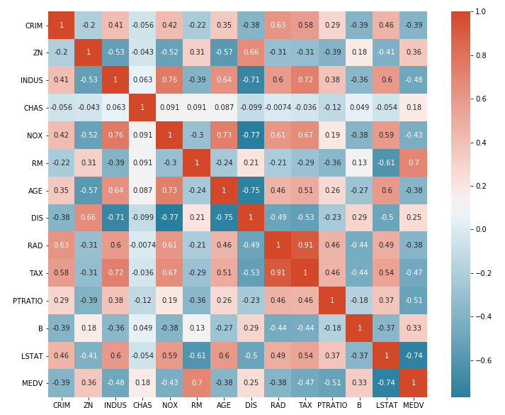
Let's see how to build this.
Seaborn heatmap | How to make a heatmap in Python Seaborn and adjust the heatmap style
The video 'Seaborn heatmap' by Kimberly Fessel clearly explains this two-step process. It shows how to compute the correlation matrix with pandas and then visualize it effectively with seaborn.
Please watch the following key segments: Correlation Matrix to Heatmap (04:05 - 05:39): This is the core part. See how .corr() is used on a DataFrame and then passed to sns.heatmap(). Choosing Colormaps (05:39 - 07:44): Learn why choosing a 'diverging' colormap like 'coolwarm' is ideal for correlation matrices. Adding Annotations (07:44 - 08:35): See how to use the annot=True parameter to display the correlation values on the heatmap, which is essential for readability.
Hands-on Practice: Creating a Correlation Heatmap
Let's use the same penguins dataset. Pandas makes calculating the correlation matrix incredibly simple with the .corr() method.
import seaborn as sns
import matplotlib.pyplot as plt
import pandas as pd


# Load the penguins dataset again
penguins = sns.load_dataset("penguins")


# Drop non-numeric columns for correlation calculation
# Note: .corr() automatically ignores non-numeric columns, but it's good practice
# to be explicit if you know you only want to correlate numeric features.
numeric_penguins = penguins.select_dtypes(include=['float64', 'int64'])


# 1. Calculate the correlation matrix
corr_matrix = numeric_penguins.corr()

print("Correlation Matrix:")
print(corr_matrix)


# 2. Visualize the correlation matrix using a heatmap
plt.figure(figsize=(8, 6)) # Set the figure size for better readability
sns.heatmap(
    corr_matrix,
    annot=True,     # Show the correlation values on the heatmap
    cmap='coolwarm',# Use a color map that's good for correlations (red=positive, blue=negative)
    fmt=".2f"       # Format the annotations to two decimal places
)
plt.title('Correlation Heatmap of Penguin Measurements')
plt.show()
When you run this code, you'll see a color-coded grid. Look for the bright red and dark blue squares (ignoring the diagonal, which is always 1). For example, you should see a strong positive correlation (around +0.87) between flipper_length_mm and body_mass_g. This makes intuitive sense: penguins with longer flippers tend to be heavier. This is another key insight, discovered in just a few lines of code.
3. Pair Plots vs. Correlation Heatmaps: Which to Use?
Both tools are essential for EDA, but they serve slightly different purposes.
| Feature | Pair Plot | Correlation Heatmap |
|---|---|---|
| Primary Use | Visual exploration of all pairwise relationships and distributions. | Quick quantitative assessment of linear relationships. |
| Strengths | - Shows non-linear patterns and clusters. - Displays individual variable distributions. - Excellent with hue for categorical analysis. |
- Scalable to many variables. - Provides a precise numeric value for correlation. - Easy to spot the strongest/weakest linear relationships. |
| Weaknesses | - Can become cluttered and slow with many variables (>10). | - Only measures linear correlation. A value of 0 doesn't rule out a strong non-linear relationship. |
A good workflow is often to start with a pair plot to get a broad visual sense of the data, then use a correlation heatmap to zoom in on the strength of the linear relationships.
Conclusion
In this lesson, you've added two powerful multivariate analysis techniques to your skillset, moving beyond single-variable analysis.
Key Takeaways:
- Pair Plots (
sns.pairplot) provide a matrix of scatter plots and histograms, giving you a comprehensive visual overview of your data's relationships and distributions. - Using the
hueparameter in a pair plot is a powerful technique to see how relationships differ across categories. - Correlation Heatmaps (
sns.heatmap(df.corr())) give you a quick, quantitative summary of the linear relationships between variables. - Customizing heatmaps with annotations (
annot=True) and appropriate colormaps (cmap='coolwarm') is crucial for creating clear and interpretable visualizations.
Preview of the next lesson:
So far in this module, we've learned how to compute summary statistics, visualize distributions, detect outliers, and now, analyze relationships between variables. We've been gathering clues. In our next lesson, we will learn how to synthesize these clues to formulate initial hypotheses about a dataset. This is where you transition from observing patterns to asking specific, testable questions that will guide your future modeling efforts.