Hello! Welcome to the final lesson in our module on regression.
So far, you've built an impressive toolkit. We started with the basics of simple and multiple linear regression, moved on to capturing non-linear patterns with polynomial regression, and most recently, you learned how to combat overfitting using the powerful regularization techniques of Ridge and Lasso regression. You've also learned how to evaluate these models using metrics like , MSE, and RMSE.
Today, we bring it all together. The goal of this lesson is to learn how to compare the performance of these different regression models on the same dataset. This is a critical skill for any data scientist, as it’s the process you'll use to select the best possible model for a real-world problem. We'll establish a systematic framework for comparison and use the metrics you've already mastered to make an evidence-based decision.
1. A Framework for Model Comparison
Before diving into code, let's establish a clear and fair process for comparing models. To ensure an "apples-to-apples" comparison, we must follow a consistent procedure:
- Prepare the Data: Start with a single dataset.
- Split the Data: Divide the data into training and testing sets. Crucially, every model must be trained on the exact same training set and evaluated on the exact same test set.
- Train the Models: Fit each of your candidate models (e.g., Linear, Polynomial, Ridge, Lasso) to the training data.
- Evaluate Performance: Calculate the same set of evaluation metrics (like and RMSE) for each model on both the training and test data.
- Compare and Select: Organize the results in a table or visualization. Analyze the scores to select the best model, considering not just the highest test score but also the balance between training and test performance to avoid overfitting.
2. A Quick Refresher on Evaluation Metrics
In a previous lesson, we covered the essential metrics for evaluating regression models. As they are central to today's lesson, let's have a quick review.
Evaluating Regression Model Metrics in Python
This resource provides concise definitions and code examples for the key regression metrics. It's a great quick reference to refresh your memory.
Please review 'Slide 2: Mean Squared Error (MSE)', 'Slide 3: Root Mean Squared Error (RMSE)', and 'Slide 4: R-squared (R²)'. Focus on the descriptions of what each metric measures and whether a higher or lower value is better.
To summarize:
- MSE (Mean Squared Error): The average of the squared differences between actual and predicted values. Lower is better.
- RMSE (Root Mean Squared Error): The square root of MSE. It's in the same unit as the target variable, making it more interpretable. Lower is better.
- R-squared (): The proportion of the variance in the target variable that is predictable from the features. It ranges from 0 to 1. Higher is better. The
.score()method in scikit-learn's regression models conveniently returns the value.
3. Comparing Models in Practice
Now let's apply our framework. We'll walk through two examples that demonstrate how to train multiple models and compare their performance.
Example 1: Comparing Linear, Polynomial, and Regularized Models
Our first resource is a comprehensive article that does an excellent job of building and comparing four different models on the same dataset. It starts simple and progressively adds complexity and regularization, comparing the results at each step.
Linear Regression with Scikit-Learn
This article, 'Linear Regression with Scikit-Learn', provides a perfect, self-contained walkthrough for our task today. You will build and evaluate several models, culminating in a final comparison.
Read through the article and its code, following the progression of models: Simple Linear Regression: Note the initial training and test scores. Polynomial Regression: Pay close attention to the for loop that iterates from degree 1 to 9. Look at the resulting table of scores. Which degree gives the best test score? Notice how the training score keeps increasing while the test score starts to drop after a certain point (overfitting). Ridge Regression: See how it's applied to the overfit polynomial model (degree 9) to improve the test score. The use of GridSearchCV here is a practical way to find a good alpha value. Lasso Regression: Finally, observe the Lasso model's performance and the final comparison table under the 'Lasso Regression' section. This table neatly summarizes the training and test scores for the regular polynomial, Ridge, and Lasso models.
The key takeaway from this exercise is the final comparison table, which looks something like this:
| Model | Score (Training) | Score (Test) |
|---|---|---|
| Reg | 0.795 | 0.747 |
| Ridge | 0.785 | 0.795 |
| Lasso | 0.786 | 0.796 |
This table clearly shows that the regularized models (Ridge and Lasso) generalize better than the unregularized high-degree polynomial model, achieving a much better score on the unseen test data.
Example 2: Comparing on a Real-World Dataset
The previous example used generated data. Let's reinforce the concept with a video that compares models on a real-world housing price dataset. This video highlights a common scenario where a simple linear regression model overfits, and regularization provides a solution.
Machine Learning Tutorial Python - 17: L1 and L2 Regularization | Lasso, Ridge Regression
This video from codebasics demonstrates the improvement gained by using regularization on a real-world dataset where a standard linear model performs poorly on the test set.
Watch the video from 07:36 to 18:50. The presenter will: First, build a LinearRegression model and show that it overfits badly (high training score, very low test score). Then, implement Lasso regression and show the significant improvement in the test score. Finally, implement Ridge regression and compare its performance, which is similar to Lasso's in this case. Focus on the score outputs for the train and test sets for each of the three models.
This example reinforces that the model comparison framework is essential for diagnosing problems like overfitting and verifying that our proposed solutions (like regularization) are actually working.
4. Visualizing and Interpreting the Results
While tables of numbers are great, visualizations can often tell a more intuitive story.
Visualizing the Fit
A simple scatter plot of your data with the regression lines of different models overlaid can immediately show which model appears to capture the underlying trend best.
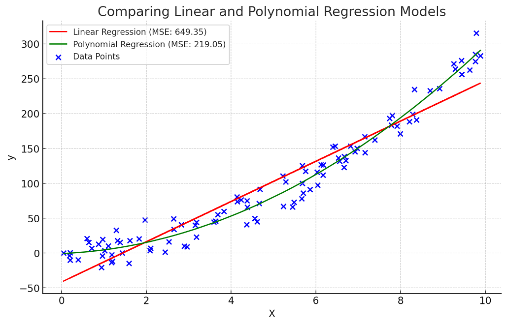
Creating a Model Comparison Dashboard
For a more comprehensive summary, you can create a "dashboard" of plots. This is a highly effective way to present your findings.

Let's break down this powerful visualization:
- Top-Left (MSE): The bar chart compares the Mean Squared Error for each model. Here, lower is better. It's easy to see which model has the lowest error.
- Top-Right (R-squared): This chart compares the score. Higher is better. It provides a complementary view to the MSE plot.
- Bottom-Left (Actual vs. Predicted): This scatter plot shows the predictions of your best model against the actual values. A perfect model would have all points lying on the red "Perfect Prediction" line. This helps you diagnose if your model has a systematic bias (e.g., always under-predicting high values).
- Bottom-Right (Regularization Path): This plot is specific to Ridge and Lasso. It shows how the model's performance () changes as you vary the regularization strength (
alpha). It's a great way to understand the effect of this hyperparameter and to see where the optimal value lies.
Presenting your results this way is a hallmark of a thorough and professional data science analysis.
Conclusion
In this lesson, you've consolidated all the skills from the regression module into a single, practical workflow. You now have a robust framework for training, evaluating, and—most importantly—comparing different regression models to select the best one for your task.
Key Takeaways:
- Systematic comparison is key: Always use the same training and test data splits for all models to ensure a fair evaluation.
- Use multiple metrics: Rely on metrics like , RMSE, and MAE to get a complete picture of model performance.
- Balance is crucial: The "best" model isn't just the one with the highest test score, but one that shows a good balance between training and test performance, indicating it generalizes well.
- Visualize your results: Use tables and plots to clearly summarize and communicate your findings. A model comparison dashboard is an excellent way to do this.
Preview of the next lesson:
We have now concluded our deep dive into regression, where the goal is to predict a continuous numerical value. We're about to switch gears and enter a new fundamental area of supervised learning: classification. In our next module, we'll tackle problems where the goal is to predict a discrete category, such as "spam" or "not spam," or "customer will churn" vs. "customer will not churn." We'll start this journey by learning about Logistic Regression, the foundational algorithm for classification.