Regularization with Ridge and Lasso

1. The Problem with Large Coefficients

Let's start by revisiting the core issue. In the previous lesson, we saw that as we increased the degree of our polynomial model, the model became more "wiggly" and complex. This complexity is mathematically represented by the model's coefficients. More complex models that are trying to capture every nuance in the training data often end up with very large coefficient values.

A large coefficient means that a small change in a feature can lead to a large change in the prediction, making the model sensitive and unstable. Regularization works by adding a "penalty" to the model's loss function for having large coefficients. This forces the model to find a balance between fitting the data well and keeping its coefficients small.

To build a strong intuition for this, let's examine a detailed example that perfectly connects to our last lesson.

2. Introducing L1 and L2 Regularization

So, how do we penalize large coefficients? There are two common ways, leading to two different regression techniques:

1. Ridge Regression (L2 Regularization): Adds a penalty equal to the sum of the squared values of the coefficients.
   • Loss = RSS + $\alpha \sum ({\text{coefficient}}_i{)}^2$
2. Lasso Regression (L1 Regularization): Adds a penalty equal to the sum of the absolute values of the coefficients.
   • Loss = RSS + $\alpha \sum |{\text{coefficient}}_i|$

Here, RSS stands for Residual Sum of Squares, which is the standard loss function for linear regression that measures the model's error. The parameter $\alpha$ (alpha), sometimes called lambda, is a hyperparameter that controls the strength of the penalty.

• If $\alpha =0$, there is no penalty, and we just have a standard linear regression model.
• As $\alpha$ increases, the penalty becomes stronger, and the model is forced to shrink its coefficients more and more.

The following video provides a clear conceptual breakdown of how these penalty terms are added to the cost function.

3. The Crucial Difference: Feature Selection

While Ridge and Lasso seem similar, the choice between a squared penalty (L2) and an absolute value penalty (L1) has a profound consequence:

• Ridge (L2) shrinks coefficients towards zero, but they rarely ever become exactly zero.
• Lasso (L1) can shrink coefficients all the way to zero, effectively removing the feature from the model.

This means Lasso can perform automatic feature selection, which is incredibly useful when you have many features and suspect that only a subset of them are truly important.

Why does this happen? The reason is geometric. Let's build the intuition with two excellent visual resources.

First, this video from StatQuest visualizes the optimization problem, showing why the L1 penalty's "sharp corners" tend to result in zeroed-out coefficients.

To reinforce this, look at the image below. It shows the contour lines of the error function (the ellipses) and the constraint region imposed by the penalty (the red shapes). The optimal solution is the point where the ellipses first touch the constraint region.

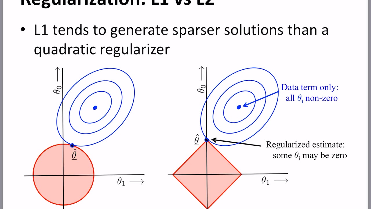
Because the Lasso constraint is a diamond, the contours will often hit one of the corners first, where one of the coefficients is zero. The Ridge constraint is a circle with no corners, so the intersection point is usually somewhere where both coefficients are non-zero.

4. Ridge and Lasso in Practice

Now let's see how this works in a practical coding example. We will follow a complete workflow where a standard linear regression model overfits, and then we'll apply Ridge and Lasso to fix it.

The following video demonstrates this entire process using a housing price dataset.

Here is a consolidated code block based on the video's example that you can run. This example uses a dataset of car features to predict their CO2 emissions. We will create polynomial features to intentionally build a complex model that overfits, then apply Ridge and Lasso.

import pandas as pd
import numpy as np
from sklearn.model_selection import train_test_split
from sklearn.preprocessing import PolynomialFeatures, StandardScaler
from sklearn.linear_model import LinearRegression, Ridge, Lasso
from sklearn.metrics import r2_score




# Load and prepare the data
# Using a common dataset from scikit-learn's documentation
url = "https://raw.githubusercontent.com/Statology/Python-Guides/main/fuel.csv"
df = pd.read_csv(url)
X = df[['ENGINESIZE', 'CYLINDERS', 'FUELCONSUMPTION_COMB']]
y = df['CO2EMISSIONS']




# Create a complex model using Polynomial Features (degree=3)
poly = PolynomialFeatures(degree=3, include_bias=False)
X_poly = poly.fit_transform(X)




# Split data and scale features
X_train, X_test, y_train, y_test = train_test_split(X_poly, y, test_size=0.3, random_state=42)
scaler = StandardScaler()
X_train_scaled = scaler.fit_transform(X_train)
X_test_scaled = scaler.transform(X_test)




# 1. Train a standard Linear Regression model (will likely overfit)
lr = LinearRegression()
lr.fit(X_train_scaled, y_train)
lr_train_score = r2_score(y_train, lr.predict(X_train_scaled))
lr_test_score = r2_score(y_test, lr.predict(X_test_scaled))

print("--- Standard Linear Regression ---")
print(f"Train R-squared: {lr_train_score:.4f}")
print(f"Test R-squared: {lr_test_score:.4f}\n")




# 2. Train a Ridge Regression model
# Alpha is the regularization strength. Higher alpha = stronger penalty.
ridge = Ridge(alpha=10) # We'll start with alpha=10
ridge.fit(X_train_scaled, y_train)
ridge_train_score = r2_score(y_train, ridge.predict(X_train_scaled))
ridge_test_score = r2_score(y_test, ridge.predict(X_test_scaled))

print("--- Ridge Regression (alpha=10) ---")
print(f"Train R-squared: {ridge_train_score:.4f}")
print(f"Test R-squared: {ridge_test_score:.4f}\n")




# 3. Train a Lasso Regression model
lasso = Lasso(alpha=1.0) # We'll start with alpha=1.0
lasso.fit(X_train_scaled, y_train)
lasso_train_score = r2_score(y_train, lasso.predict(X_train_scaled))
lasso_test_score = r2_score(y_test, lasso.predict(X_test_scaled))
num_zero_coeffs = np.sum(lasso.coef_ == 0)

print("--- Lasso Regression (alpha=1.0) ---")
print(f"Train R-squared: {lasso_train_score:.4f}")
print(f"Test R-squared: {lasso_test_score:.4f}")
print(f"Number of coefficients set to zero: {num_zero_coeffs} out of {X_train_scaled.shape[1]}\n")

When you run this code, you should notice that the standard LinearRegression model has a very high training R-squared but a much lower test R-squared, indicating overfitting. Both Ridge and Lasso should have more balanced scores, showing they generalize better. Notice how Lasso sets many coefficients to zero, effectively simplifying the model.

5. Visualizing the Impact of Alpha

The choice of alpha is critical. A powerful way to understand its effect is to plot the value of each coefficient as alpha increases. This is known as a coefficient path or trace plot.

These plots are the definitive visual summary of the behavior of Ridge and Lasso. They show you exactly which features Lasso deems unimportant first and how Ridge treats all features more uniformly.

The optimal value of alpha is typically found using cross-validation. We will cover the tools for this systematic hyperparameter tuning, like GridSearchCV, in a future module.

Conclusion

You've now learned one of the most important concepts for building robust machine learning models. Regularization is a standard part of the modern data scientist's toolkit for creating models that are not only accurate but also stable and generalizable.

Key Takeaways:

• Regularization is a technique to prevent overfitting by adding a penalty for large coefficients to the model's loss function.
• Ridge Regression (L2) uses a squared penalty. It shrinks coefficients towards zero, which is effective at handling multicollinearity and reducing model complexity.
• Lasso Regression (L1) uses an absolute value penalty. It can shrink coefficients all the way to zero, performing automatic feature selection.
• The alpha hyperparameter controls the strength of the regularization. A larger alpha results in smaller coefficients and a simpler model.

Preview of the next lesson:

So far in this module, we've built several types of regression models: simple linear, multiple linear, polynomial, Ridge, and Lasso. But how do we decide which one is truly the best for our specific problem? In the next lesson, you will learn how to compare the performance of different regression models on the same dataset, using a structured approach to select the most effective model.