Multiple Linear Regression: Model Fitting and Multicollinearity Assessment

1. From One Feature to Many: Multiple Linear Regression

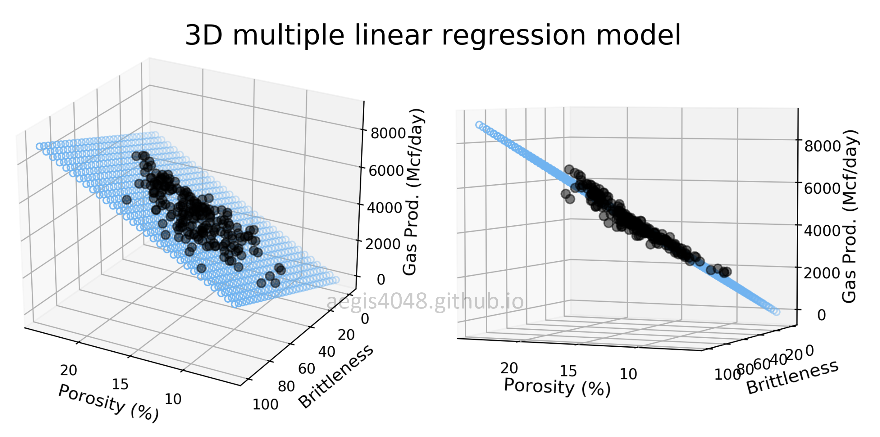
Multiple Linear Regression (MLR) is a natural extension of the simple linear regression you've already learned. Instead of modeling a line, we are now modeling a plane (with two features) or a hyperplane (with more than two features) that best fits the data.

The equation simply expands to include more variables:

• Simple Linear Regression: $\text{price}=b_0+b_1\times \text{area}$
• Multiple Linear Regression: $\text{price}=b_0+b_1\times \text{area}+b_2\times \text{bedrooms}+b_3\times \text{age}$

Here, $b_0$ is still the intercept, and $b_1,b_2,b_3$ are the coefficients for each feature. Each coefficient $b_i$ now represents the change in the target variable for a one-unit change in feature $x_i$, holding all other features constant.

This image shows what this looks like with two features. The model is no longer a line, but a flat plane slicing through the 3D space of data points.

Let's see how to implement this in Python. The great news is that scikit-learn makes this transition incredibly easy.

As you saw, the core scikit-learn workflow doesn't change. You prepare your feature matrix X (which now has multiple columns) and your target vector y, and then call model.fit(X, y).

2. The Problem of Redundant Features: Multicollinearity

Now that you can add many features to your model, a new question arises: what happens if the features themselves are correlated? For example, what if we have features for both a person's age and their years of work experience? These two are likely to be highly correlated.

This situation is called multicollinearity, and it can cause problems, particularly with interpreting your model's coefficients.

To build a strong intuition for what multicollinearity is and why it's a problem, the following video offers an excellent deep dive.

Key Effects of Multicollinearity:

• Unreliable Coefficients: The coefficient estimates can swing wildly depending on which other variables are in the model. A coefficient might even flip its sign (e.g., from positive to negative) when a correlated feature is added.
• Inflated Standard Errors: This makes it difficult to determine which features are statistically significant. A very important feature might appear insignificant simply because it's correlated with another feature.
• Prediction is Often Unaffected: Importantly, multicollinearity often doesn't hurt the model's overall predictive accuracy. If your only goal is to make predictions, you might not need to worry about it. However, if you want to understand the individual impact of each feature (which is a core part of data science), you must address it.

3. Detecting and Handling Multicollinearity in Python

The most common and robust way to measure multicollinearity is by using the Variance Inflation Factor (VIF).

The VIF for a feature measures how much the variance of its estimated coefficient is increased due to collinearity with other features.

Rules of thumb for interpreting VIF:

• VIF = 1: No correlation.
• 1 < VIF < 5: Moderate correlation, often not a problem.
• VIF > 5 or 10: High correlation, which is likely problematic and should be inspected.

Let's put this into practice. We'll use the California Housing dataset and calculate the VIF for each feature.

Here's the essential code snippet from the article for calculating VIF. You'll need to have the statsmodels library installed (pip install statsmodels).

import pandas as pd
from sklearn.datasets import fetch_california_housing
from statsmodels.stats.outliers_influence import variance_inflation_factor




# Load the dataset
housing = fetch_california_housing()
X = pd.DataFrame(housing.data, columns=housing.feature_names)




# Calculate VIF for each feature
vif_data = pd.DataFrame()
vif_data["Feature"] = X.columns
vif_data["VIF"] = [variance_inflation_factor(X.values, i) for i in range(X.shape[1])]

print(vif_data)

After running this code, you'd find features with high VIF scores. A common strategy to resolve this is to remove one of the features from a highly correlated pair and then refit the model. For instance, since Latitude and Longitude are highly correlated and provide similar location information, you might decide to keep only one, or create a new feature from them. Similarly, you would likely remove AveBedrms because it is highly correlated with AveRooms.

Conclusion

You've made significant progress today. You've moved beyond simple models and can now leverage multiple features to make predictions, and you're equipped to handle the important challenge of multicollinearity.

Key Takeaways:

• Multiple Linear Regression extends simple linear regression by using multiple features to predict a target variable. The scikit-learn implementation remains simple: model.fit(X, y).
• Multicollinearity occurs when independent variables in your model are highly correlated with each other.
• This correlation makes it difficult to interpret individual feature coefficients, as their estimates become unstable and standard errors get inflated.
• Variance Inflation Factor (VIF) is the standard method for detecting multicollinearity. A VIF value above 5 or 10 is a red flag.
• The most common way to handle multicollinearity is to remove one of the highly correlated features and refit the model.

Preview of the next lesson:

Our linear models have so far assumed a straight-line (or flat-plane) relationship between features and the target. But what if the relationship is curved? In our next lesson, you will learn to implement polynomial regression to model these non-linear relationships, giving you another powerful tool for your modeling toolkit.